I created a new simulation project called 'NACA 0012 Verification':
To verify the setup to be used in analysing aerodynamic bodies
More of my public projects can be found here.
I created a new simulation project called 'NACA 0012 Verification':
To verify the setup to be used in analysing aerodynamic bodies
More of my public projects can be found here.
We are a a team of students working on a project run by the Institution of Mechanical Engineers called the UAS challenge. This challenges gives teams the opportunity to design, build test and compete their solution to a problem in the form of an unmanned aerial vehicle. Our team is excited to be sponsored by SimScale and are determined to show how we use SimScale to be successful in this challenge.
It is a common for users to believe that once a software has been validated to produce realistic results, that a user can simply mesh and simulate their designs, and be returned with accurate results. Unfortunately this is rarely the case, and regardless of your experience level, you could be subject to poor results without knowing unless a verification of your methodology had taken place. In terms of cost, you could design something that works on paper, but due to poor analysis, the product does not work and is only discovered at the end of development.
The most responsible approach to development is understanding the validated results, verifying your own setup, and relying on the methodology developed to give good results through the development of the product, whilst periodically verifying results.
Therefore, this project will set about developing the methodology for reliable results, observe what settings are sensitive to sensible results, and what kind of accuracy can be achieved using a realistic mesh. By a realistic mesh, we mean a mesh that, at density, could be achievable in 3D full wing or even full aircraft scale.
Discretisation error is a common and well-known cause of inaccurate results, and a well-known solution is to perform a mesh independence study, this, in essence, determines at what point mesh fineness stops dramatically effecting results and therefore any finer would be a waste of computational resources. It is, therefore, necessary to take several meshes and observe the lift and drag results on these meshes.
With lift remaining fairly constant at above 97% accurate, it is safe to say that it is already mesh independent, however, drag being very small values, the smallest change in accuracy a greater percentage effect. Therefore, throughout the study, it significantly increased from approximately 80% accurate up to approximately 97%. For efficiency sake, when 3D shapes start getting mesh, 90% accuracy from the experimental result could be afforded.
The above figure of the used mesh shows that a significant amount of layering was required as to not cause the mesh size in terms of number of cells to go too high, as a result the cells at the wall have an extremely high aspect ratio, whereas the cells at the final layer have a low aspect ratio, and approximately the same volume as the surrounding mesh. Y+ was reduced to around 1 so that the viscous sub layer could also be resolved, this was all obtained using the standard wall model.
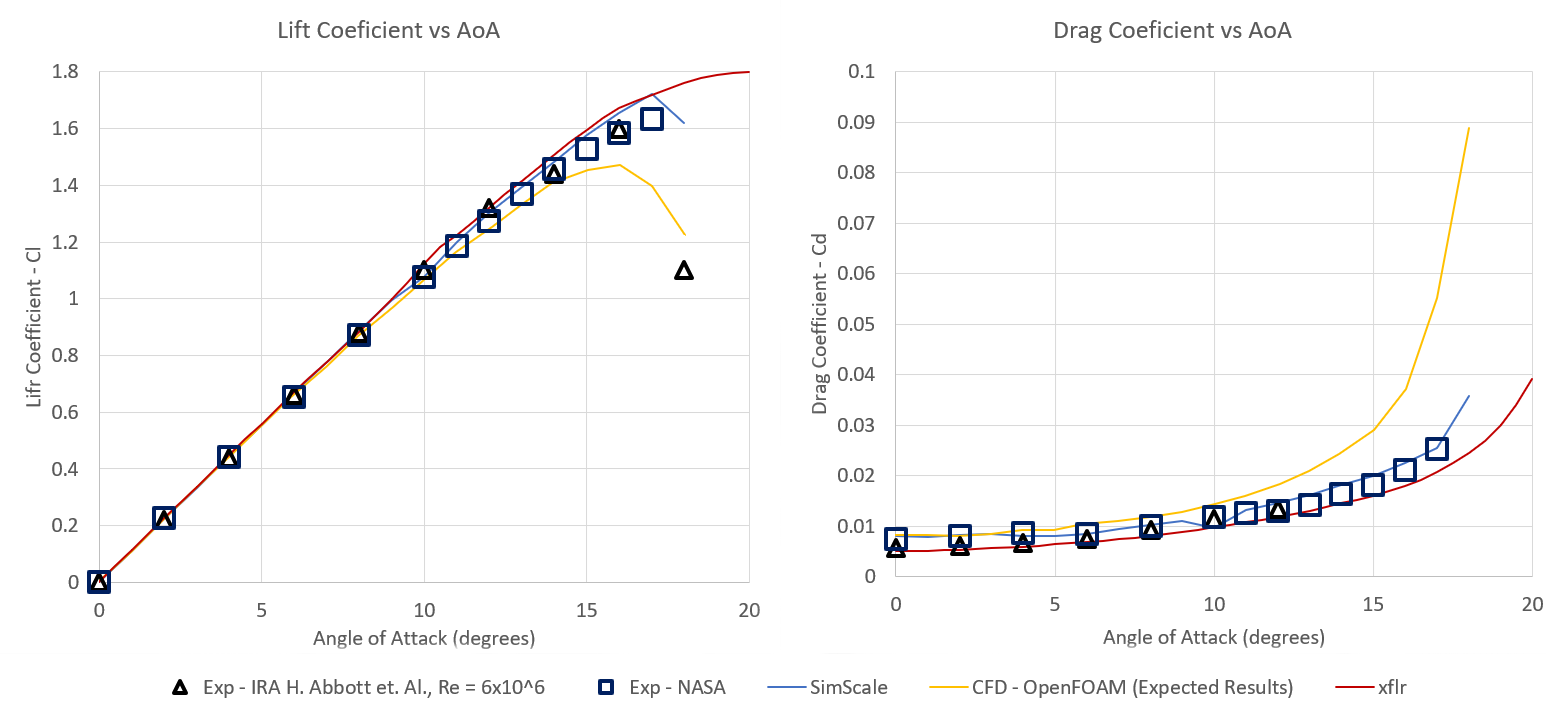
To gauge accuracy, results were obtained from two sources, the first, (IRA H. Abbott and Albert E. Von Doenhoff, 1958) where experimental results for both lift and drag were taken the second, a more recent paper (Sorribes Palmer et al., 2018) provided a clear graph containing experimental results originally from NASA, but more importantly, an openFOAM validation of several aerofoils including the selected NACA 0012 to provide an expected minimum accuracy of which we could achieve.
The expected results were obtained using the K-omega SST model, as were our results on the SimScale platform, this model is known for its accuracy in such an application and provides good wall modelling across a large range. As most RANS models, however, its accuracy is expected to drop off as the stall is approached due to the accuracy that is available when flow separation occurs. The solution to this would be to use a transient model where even URANS is known to improve this accuracy. This can be visualised in the comparison below of an aerofoil at an AoA of 20 degrees, where the first is solved as a steady problem the second transiently.
The results show that the methodology, solver and mesh used exceeded expectations pretty much everywhere, with an exception at 18 degrees where the drop in lift reported in (IRA H. Abbott and Albert E. Von Doenhoff, 1958) were achieved closer in the expected results (Sorribes Palmer et al., 2018) whereas, leading up to the point it could be argued we continue to exceed the expected results. Most significantly to note is the continued accuracy achieved in drag calculations.
Results were surprisingly sensitive to certain numerical schemes, where they made the difference between a failed validation and perfect validation. The reason is that higher order schemes are less susceptible to error when a coarse mesh is used, and the default Bounded Gauss Upwind (first order) divergence scheme for velocity was the sensitive scheme. Despite the name, Gauss linearUpwind is a second order (Tobias Holzmann, 2017) scheme, and produced the validation results shown above.
In addition to this, smooth reached steady state very slowly and sometimes results were mistaken to be converged since the change was very minimal across iterations, PBiCG remained stable and converged faster in most cases.
The SimScale platform as originally proven by Ali Arafat, validate well for lift, and now shown, also validates well for drag values. The numerics, mesh and boundary conditions required to setup such a case have been verified to reproduce results that have been proven time and time again to validate well. We can now move forward in confidence to be able to reproduce results similar to those obtained experimentally and know the limitations of the setup and where extra allowances need to be made to tolerance (nearing stall for example).
IRA H. Abbott and Albert E. Von Doenhoff (1958) Theory of Wing Sections. 2nd edn. New York: Dover Publications.
Sorribes Palmer, F., Donisi, L., Pindado Carrion, S., Gómez Ortega, O. and Ogueta Gutiérrez, M. (2018) Towards an airfoil catalogue for wind turbine blades at IDR/UPM Institute with OpenFOAM.
Tobias Holzmann (2017) Numerical Schemes. (Accessed: 01/11/2018).
Thanks for sharing.I found a lot of interesting information here. A really good post, very thankful and hopeful that you will write many more posts like this one.
Great work.
How did you do the meshes that you used?
Hi @Filiptheking, the mesh was a small effort, unfortunately, to keep layers inflated at sharp edges I refined a small fillet that would be insignificant to results. I then downloaded the mesh, used the OpenFOAM utility extrudeMesh to create it in 2D from a side face, I then re-uploaded it.
Best,
Darren
Hi Darren,
I am trying to figure out which simulation runs that you drew your data from to make both your Lift Coefficient vs AoA and your Drag Coefficient vs AoA plots…
For instance, there are so many sim runs for AoA 10 degrees, which one did you use?
Dale
@DaleKramer take the first batch of tests, the ones at the end with long names were mesh independence tests and random tests (this is still my testing ground for aerofoils),
Best,
Darren
Fair enough, but there are still 10 converged runs on simulation ‘AoA10’. Do I assume that you averaged the results of those 10 runs or do I have to find the one that ‘I think’ mostly closely matches the data on the plot 
@DaleKramer, I just sampled some of my simulations, and yer fair point, there are cartloads of runs. If I find time this week I will clean the project up and keep a copy private, I suppose for now just assume the last run but take it with a pinch of salt.
Sorry, I’ll see what I can do.
Darren
Also, are you using that last iteration parameter value in the run for your runs’ result value?
Personally, I try to use values that are 1% stable over a significant number of iterations and then specify that range…
For instance, I look at the force plots over time, select a lowest point value near the end time, then I multiply that value by 1.01, use that 1.01 scaled value to find out the last iteration that was not above it (this becomes the start of 1% range and the end is the last iteration time).
Then I specify my actual value as 1.005 times the lowest value in the range and the result would be this 1.005 scaled value +/- 0.5%…
No I don’t report any error and basically use the last timestep. Typically after or near stall, if the results are unstable to the point that I cannot draw a steady-state conclusion, then I do not report as then it should be analysed in transient. So what you see in the graphs are likely to last iteration values.
Best,
Darren
When I see stable but fluctuating results, I try to see if the best fit ‘center line’ of the fluctuations is stable to 1%… stable and use the ‘centerline’ middle value for my result value with a +/-% of the peaks of the fluctuation in the range… (this assumes that the fluctuations are themselves relatively small and stable).
Actually, just a prominent note in post 1 about which Sims and Runs that the data came from and the fact that the data represents results from the last iteration of each run would be good for me…
I kinda like seeing the way you converged onto such apparently fine results ![]()
Darren, do you have a link to the NASA experimental results that you plot 
Hi @DaleKramer, I will look in my dissertation to find the source, I think it was the same source the ‘openfoam expected results’ came from, and if so will be a paper (that you may have to buy) but NASA have published results on their validation page, that I would expect to be the same:
https://turbmodels.larc.nasa.gov/naca0012_val.html
I will update with the paper when I find it in the reference section.
Best,
Darren
Yes, but that link is for 6 million RE and your 2 meter chord at 80 mps is ~12 million RE…
Either you did not use that link data or perhaps you should have used 40 mps?
EDIT: And are you using the same air density and viscosity as the NASA data?
If that were so, why are the NASA and OpenFoam Expected results different?
@DaleKramer, Text edited to explicitly say where the results came from to avoid confusion.
Best,
Darren
Sorry, I was getting messed up with other the domains and meshes there, and yes you have correctly pictured the mesh for sim run AoA10 (which is the case of interest for me as that is where your CFD data to compare came from)… My fumble