Sports Aerodynamics Workshop: Session 1 Homework
Recording
NOTE:
Rather than contacting our support, please try to put your query/ies regarding problems in setting up your simulation or having failed simulation runs under this forum post. This will assure much faster solution to your problem/s and also help others to tackle similar kind of problem in case they have one. Thank you for your understanding. Good luck! ![]()
Homework Submission
Submitting all three homework assignments will entitle you to a certificate of participation.
Homework 2 - Deadline: 6th March 2017, 12pm
Introduction
Having been familiarized with the Simscale platform, the user can now follow this tutorial which aims at providing hands-on experience with the platform. Essentially, a parametric study generic to ski-jumping aerodynamic analysis is the central topic of this homework assignment. The user is enabled to explore the end-to-end (geometry upload to post-processing) approach of the Simscale platform.
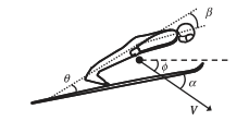
Now to provide some basic background about the mechanics of ski-jumping dynamics, the equations of motion of the ski-jumper [1]:
![]()
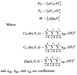
the lift, drag and moment can be calculated as follows:
The equations might look tedious to solve. This is where the power of Computational Fluid Dynamics (CFD) comes into play. The lift (FL) and drag forces (FD) may be evaluated from the simulation results and be directly plugged into the equations of motion of the ski-jumper.
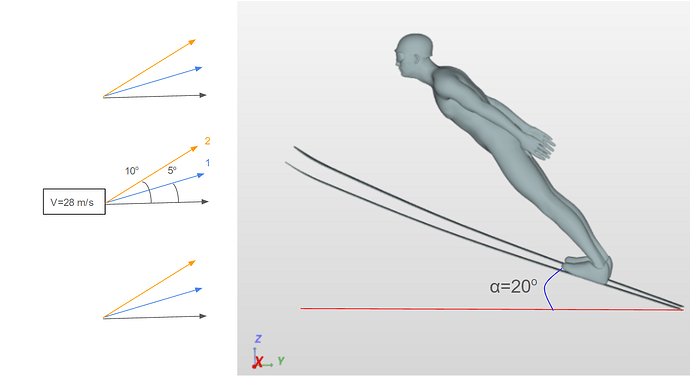
The demonstration session for Ski-jump Aerodynamics considered an angle of attack of 20o at a velocity of 28 m/s. As promised, the task for this assignment is to evaluate the lift and drag forces at different angles of attack (α). You are free to assign an angle of attack within the range of (1o,10o).(*)
(*)Please Note: This range is intended to operate within safe bounds of stall, which in turn would lead to the strong vortices and possibly lead to numerical instabilities in the solver. The more curious users are free to explore!
In physical terms this range would correspond an angle of attack of (20o,30o) based on the fact that the baseline geometry we are using is inclined at an angle of 20o.
Exercise
Investigate the influence of the angle of attack for two different angles between 0° and 10°.
For this tutorial, angles of attack: 5o and 10o have been selected with an inflow velocity of 28 m/s.
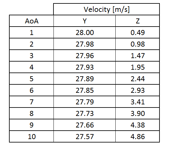
The velocity components in the y- and z- directions can be calculated as follows:
Example 1:
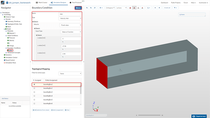
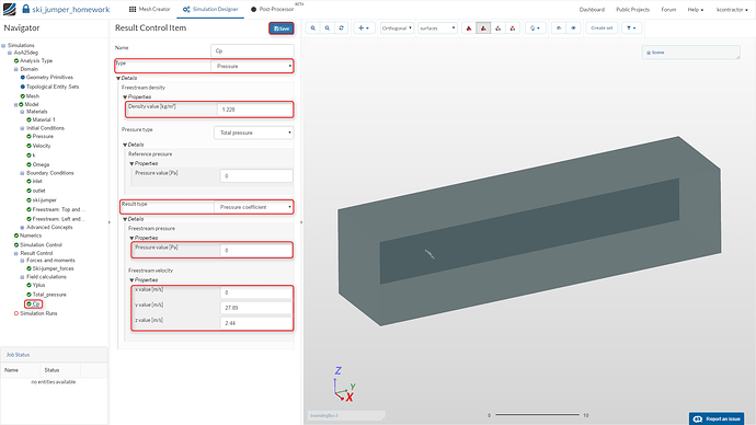
Y velocity: 28 x cos(5)= 27.89 m/s
Z velocity: 28 x sin(5)= 2.44 m/s
Example 2:
Y velocity: 28 x cos(10)= 27.57 m/s
Z velocity: 28 x sin(10)= 4.86 m/s
But feel free to choose a different degree from this list:
Deliverables:
- Link to your simulation project for your first Angle of Attack.
- Link to your simulation project for your second Angle of Attack.
- Evaluation of Lift and Drag Forces from the two simulations. Which Angle of Attack would be your choice? Please justify.
- Post processing Total Pressure slices and Velocity streamlines (optional: with comments on the physics)
Handout Project:
This project can be used as a starting point for your simulation.
Mesh Generation
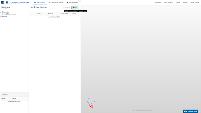
Once the geometry has been imported into the platform, we proceed to the mesh generation. In the navigator pane, please select Meshes button and click on New.
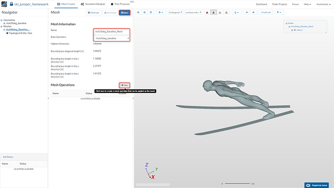
The platform now provides you with the option to select the geometry you would like to work with. This option comes in handy when a parametric study with geometric variations is needed. In this homework exercise, we will work with a single geometry. Please assign an appropriate name for your mesh and select the geometry, AoA20deg_Baseline_Mesh.
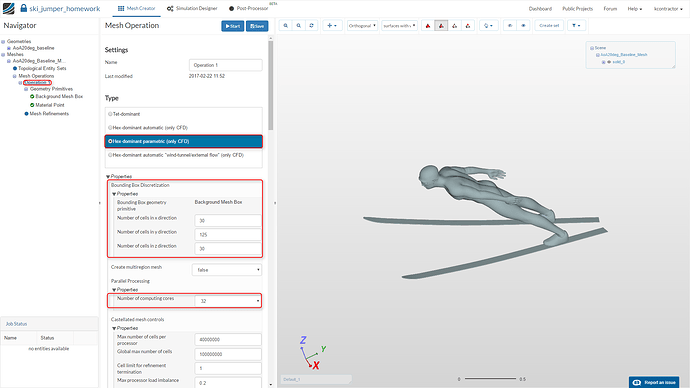
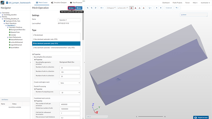
We will be using the Hex-dominant parametric (only CFD) option for this homework. This approach provides a good user-control over the mesh. Please enter the number of cells in the x-, y- and z- directions as per the image below. This is done to have a uniform mesh in all directions.
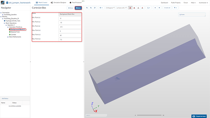
Min. Point (x )= -6
Min. Point (y) = -10
Min. Point (z) = -4.5
Max. Point (x) = 6
Max. Point (y) = 40
Max. Point (z) = 7.5
The Background Mesh Box is the domain on which the calculations will be made. It is assigned such that it does not interfere with the physics of the simulation. For example, it is made long enough in the downstream (+y) direction to minimize the influence of wake vortices on the outflow.
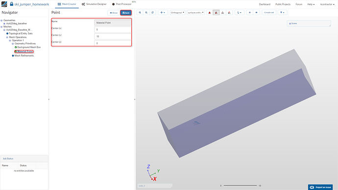
The introduction of a Background Mesh Box splits the domain into two parts; inside the ski-jumper and outside the ski-jumper. The material point decides the part of domain on which the calculations will be made. This tutorial aims at simulating the external flow around the ski-jumper, hence the Material point can be placed anywhere outside the ski-jumper (but within the bounds of the Background Mesh Box). We select our Material Point at the location: (0,10,0).
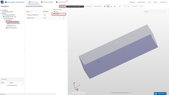
Now, we proceed to add another geometry primitive to our domain. Please select Geometry Primitives in the Navigation pane and click on New. Then select the option, Cylinder.
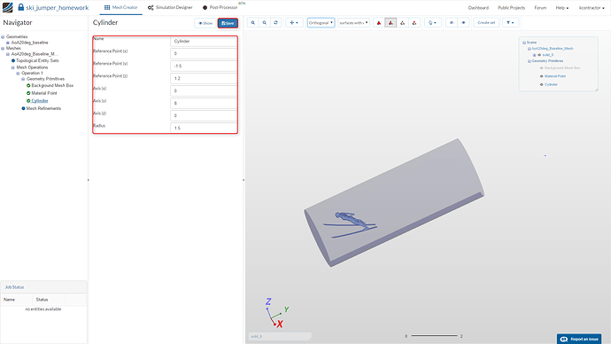
This Cylinder is intended for further mesh refinement in the wake region of the ski-jumper. The size and position of the Cylinder can be adjusted as per the required fidelity level of the simulation.
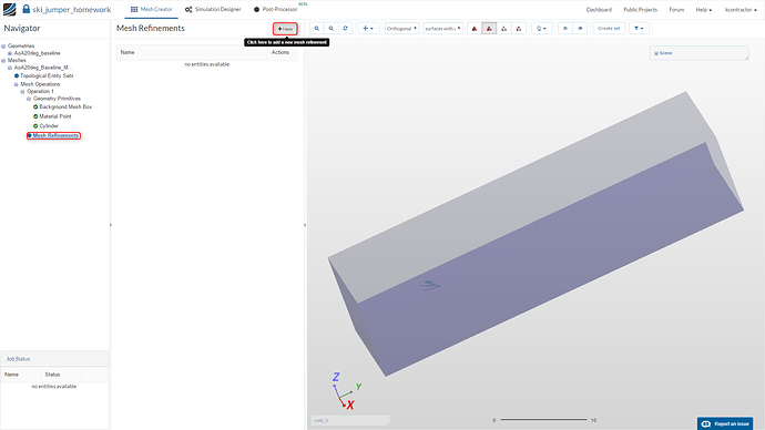
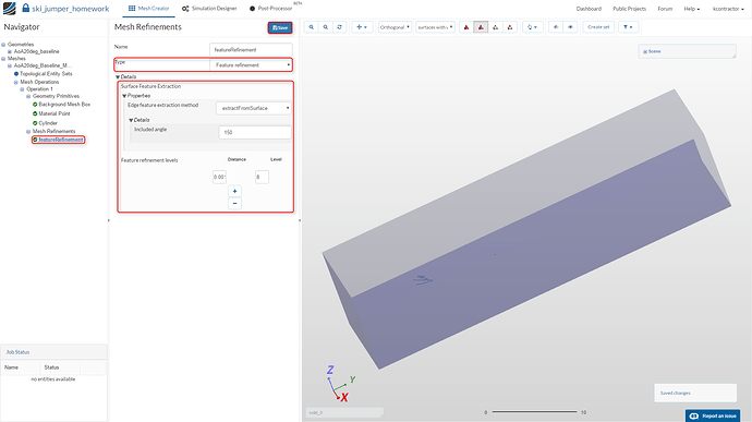
Mesh refinements are crucial to the convergence and accuracy of any CFD simulation. As a next step, we move onto mesh refinements by selecting Mesh Refinements in the Navigation pane and followed by clicking on New.
Please Note: After creating a new mesh refinement, select the Type and click on Save.
Feature Refinement allows you to create a finer mesh close to edges. It extracts the edges from the surfaces and refines the mesh as defined in the “Feature Refinement Levels” panel.
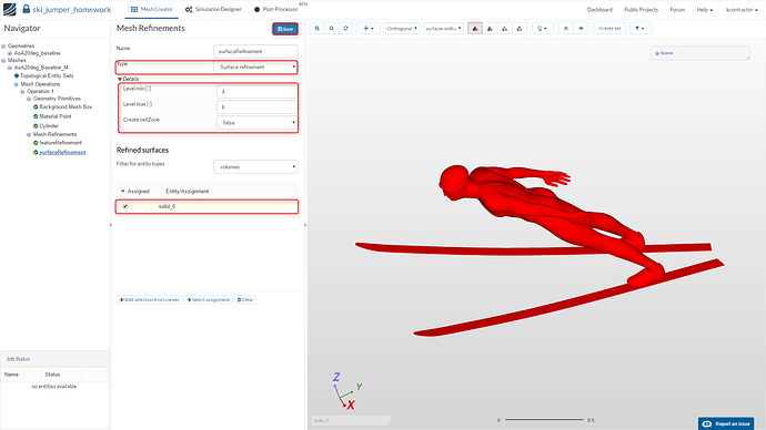
A Surface Refinement can be created for faces or solids. In both cases, the mesh will be refined near the surface of the selected object. Please implement a surface refinement as shown in the below image.
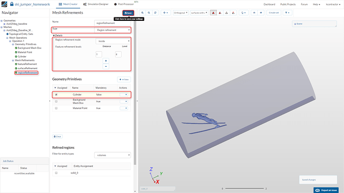
Region Refinement provides the option to refine your mesh in a pre-specified region. This region may be a solid body or a geometry primitive. We had previously defined a cylinder, which will now serve the purpose of region refinement. Please make sure that the Region refinement mode is set to inside. Select Cylinder from the Geometry Primitives as the region to be refined.
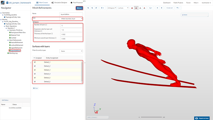
The Inflate Boundary Layer option enables you to define prism layers on the selected faces in order to efficiently capture the boundary layer. The Inflate Boundary Layer is especially important in this homework assignment since we have strong re-circulation and vortices in the wake of the ski-jumper. The y+ values are limited by this refinement. Please add a new refinement and select the Type as Inflate Boundary Layer. Next, click on Save.
Number of layers = 5
Expansion ratio for layer cell thickness = 1.2
Thickness of the final layer = 0.005
Minimum overall layer thickness = 0.002
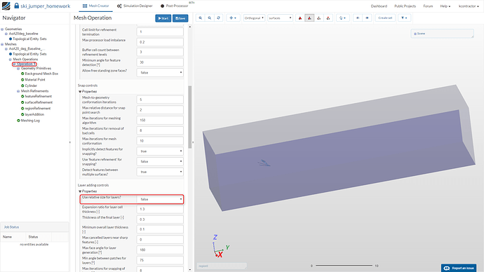
The cell sizes defined in Thickness of the final layer and Minimum overall layer thickness are absolute. In order for the mesh generator to know this, please navigate to the Operation 1 in the Navigation pane and set Use relative size for layers to False.
You are now ready to begin the mesh generation. Please select Operation 1 from the Navigation pane and click on Start.
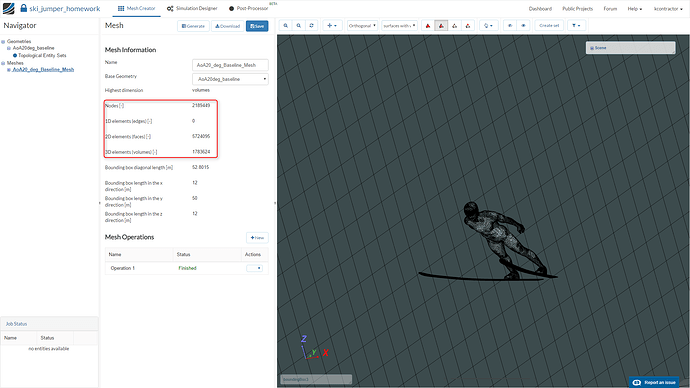
The mesh can now be visualized on the platform:
The more enthusiastic users can also qualitatively and quantitatively analyse the mesh in more detail with mesh clips and the meshing log, respectively.
Simulation Setup
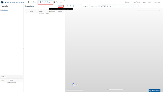
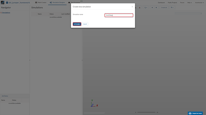
The mesh now been setup and satisfactorily analysed. The next step in your workflow is to move into the Simulation Designer. To create a new simulation, please click on New.
Please assign a name to your simulation and click Create.
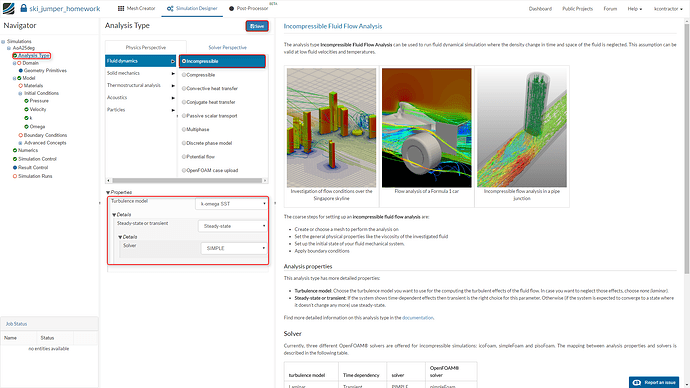
Based on the fact that the maximum speeds attained by the ski-jumper are well below Mach 0.3 (a thumb-rule for compressibility), Incompressible can be selected as the Analysis Type.
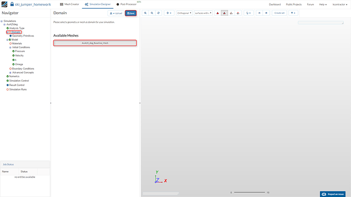
Proceeding to Domain selection, you can select the mesh on which you want the simulation to be performed. This is particularly productive when you want to work with different meshes.
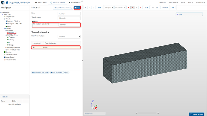
The working fluid is now assigned. Please enter the value of Kinematic Viscosity for air and select the volumetric Region on which the material needs to be assigned.
The initial conditions are assigned to the whole domain at the start of a simulation. During a simulation, the solver tries to converge the solution fields after taking these initial condition values as a starting point. Therefore, it is important to assign best guesses or analytical solutions as initial conditions when possible.
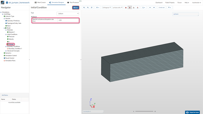
We assume a low turbulence intensity of air (I=5%=0.05) for our simulation. The values of Turbulence Kinetic Energy (K) and Omega (ω) can be calculated (Formulae)*:
Turbulence Kinetic Energy (K) = 2.94
Omega (ω) = 4.28
Please feed in the values of K and omega into their respective positions in the Navigation Pane.
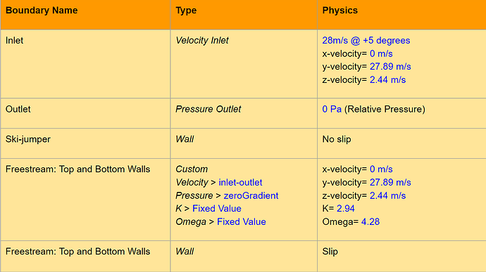
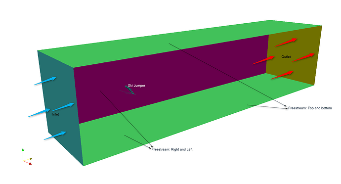
The overview of the physics setup is as follows:
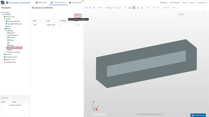
You may now proceed to setup the physics of the simulation. To create a new boundary condition, please select Boundary Conditions in the Navigation plane and click on New.
The inlet boundary condition can be created as follows:
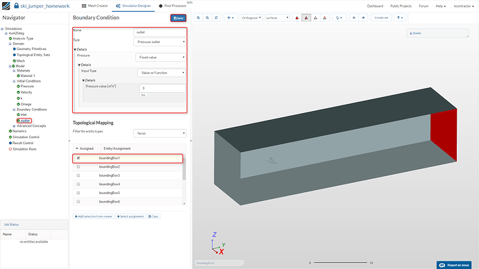
Please create a New Boundary Condition. The outlet boundary condition can be created as follows:
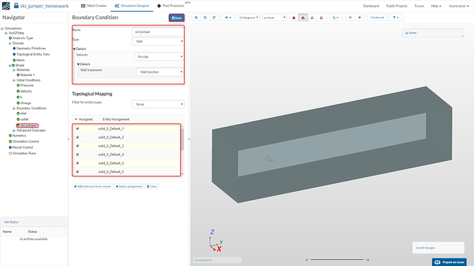
Please create a New Boundary Condition. The ski-jumper boundary condition can be created as follows:
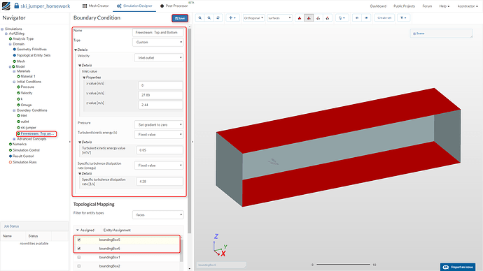
This boundary condition, known as freestream: Top and Bottom, is a bit tricky. Owing to the fact that the inlet velocity is inclined in the YZ-direction, there will be a component of velocity which exits the domain from the top and bottom bounds of the domain. Hence, the standard “Slip Wall” boundary condition is not advisable in this case. In order to circumvent this, you can select a Custom boundary condition and assign Inlet-Outlet to the Velocity field.
Please create a New Boundary Condition. The freestream: Top and Bottom boundary condition can be created as follows:
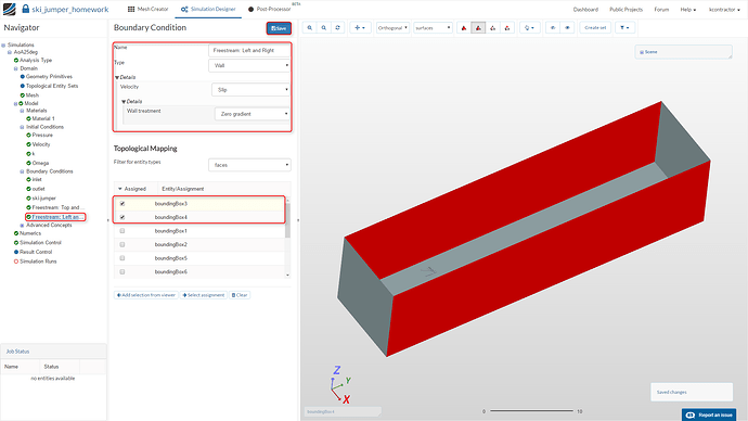
The freestream: Right and Left can be treated as a Slip wall since there is no component of inflow in the x-direction. Please create a New Boundary Condition. The freestream: Right and Left boundary condition can be created as follows:
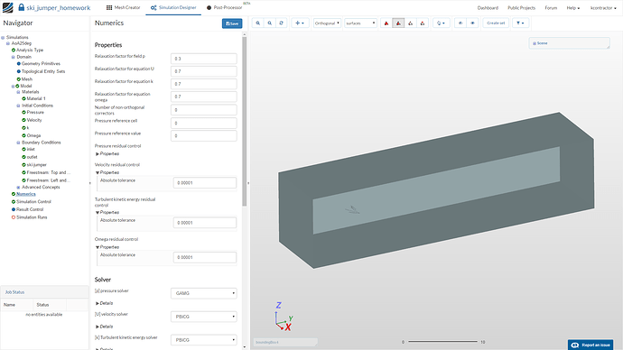
The Numerics on the platform have been optimized and do not need to be changed for this simulation. You could analyse them by selecting Numerics in the Navigation pane :
The Simulation Control provides user-control over the simulation. You can increase the Number of computing cores to 32 and Maximum runtime to 8000s.
Please note: The End time value represents the computation time and Maximum runtime represents the wall clock time (real time!)
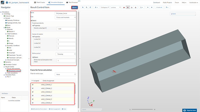
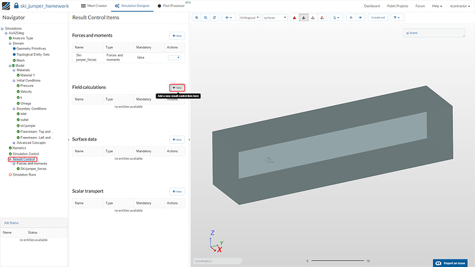
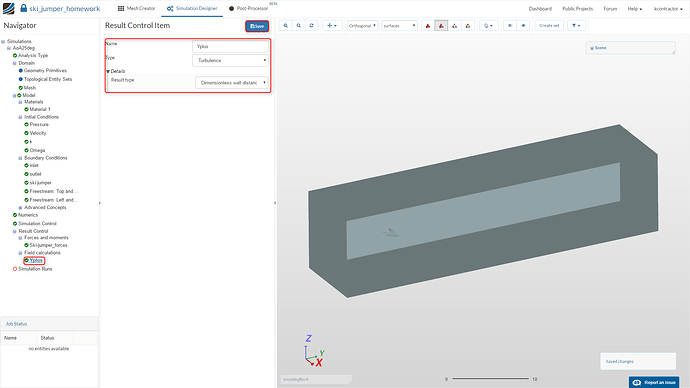
For the purpose of accurate verification or validation of the results, additional solution fields need to be post-processed. The platform provides a Result Control panel to serve this purpose. The additional Result Control Items (solution fields) can be setup and exported as follows:
<img src=“/forum/uploads/default/original/2X/8/820b103ff92c22397c7f265723f19cbaed6b77a0.png” alt=“sports aerodynamics workshop homework step-by-step tutorial, result verification validation” title=“Click “New” to add a new result control item” width=“690” height=“388”>
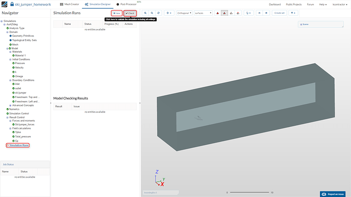
You are now almost ready to start your simulation run. Please navigate to Simulation Runs in the Navigation pane and Check the simulation setup. If there is no error, please create a new run by clicking on New.
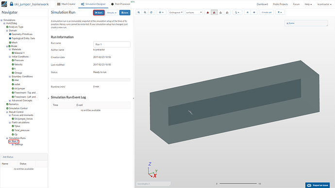
Please click on Start to begin your simulation run.
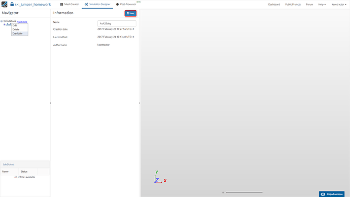
To create the proceeding simulations, you can simply duplicate the simulation setup by right clicking on the simulation you would like to duplicate and press Duplicate.
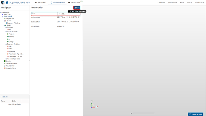
Please feed-in the name of your new simulation and click on Save.
Post-Processing
Please navigate to the Post-Processor in the workflow.
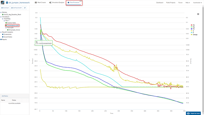
The Convergence Plot:
The residual convergence can be visualized by selecting the Convergence Plot in the Navigation pane.
The Force Plot:
The force plot over the jumper can be visualized by selecting ski_jumper_forces. The unwanted forces and moments can be deselected by clicking them on the right edge of the force plot.
As a general best practice for steady state flow problems, it is advisable to average the flow properties, such as Forces, over the final timesteps.
The lift and drag forces on the ski-jumper can be evaluated from the ski_jumper_forces plot:
Lift = Pressure force z + Viscous force z
Drag = Pressure force y + Viscous force y
Slices:
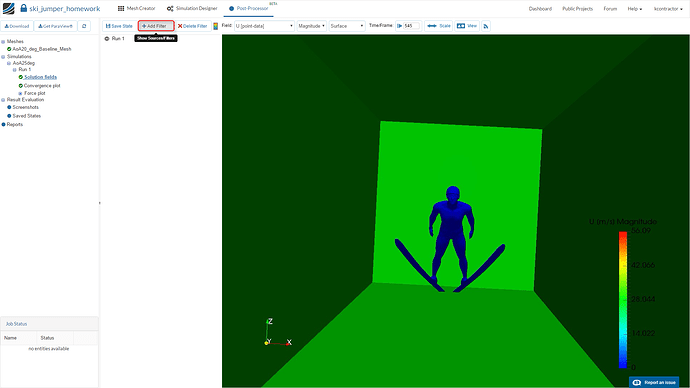
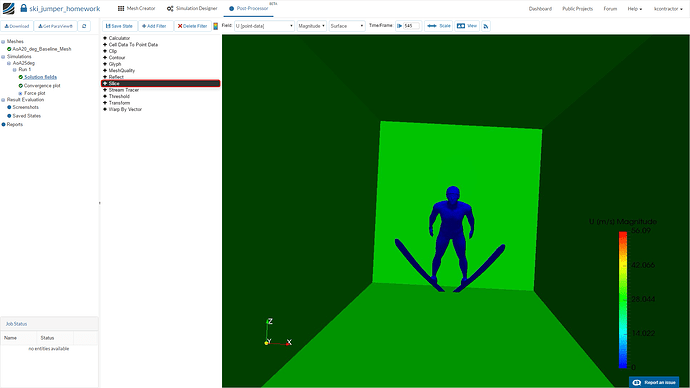
The solution fields may be visualized on the platform by utilizing filters. Please select Solution fields in the Navigation pane and select the Cell arrays you would like to analyse. Next, move to your final timestep in the window time/frame. You are free to toggle your view with the View window.
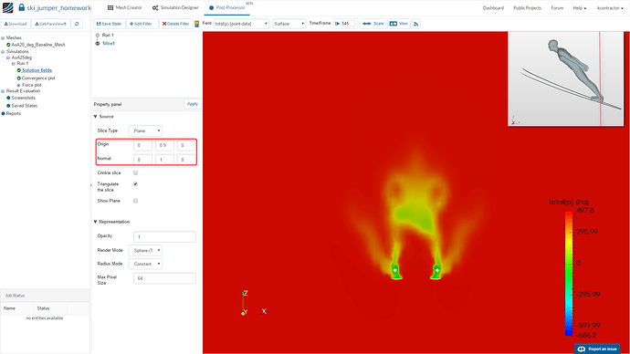
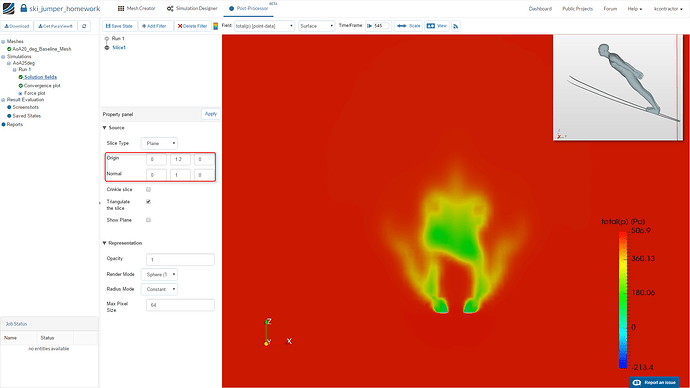
Now, to create a slice click on Add filter and select Slice.
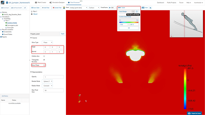
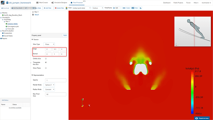
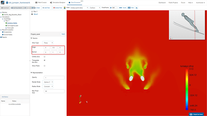
The location of the slice can be customized in the windows, Normal and Origin. Please make sure to deselect Show plane. The data can be auto-scaled by utilizing the Auto-range in the Scale window.
Streamlines:
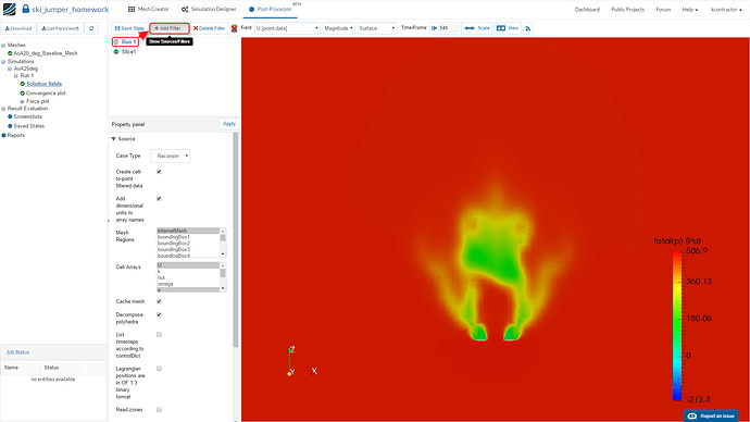
To create a new filter, select your simulation run (Run 1 in this case) and Add filter.
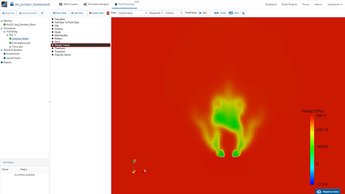
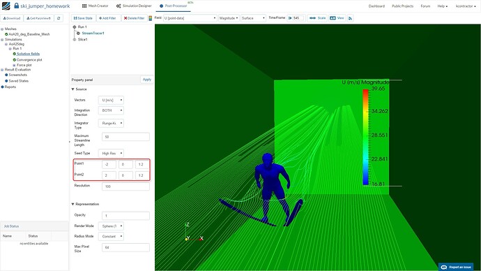
Please select Stream tracer from the list of filters.
To have a clearer view of the 3D streamlines we analyse streamlines categorically by setting the Seed Type as High resolution line. The location can be set with the tabs Point 1 and Point 2.
The user is also free to analyse the results locally by downloading it to their system. An opensource post-processor, Paraview, can be downloaded here.
Thank you for your attention and happy simulating!

