NOTE: This tutorial was updated on 10/2016 to match the updated version of the platform
If you would like to watch the fourth session of the Drone Workshop again or in the case you missed it, you can access the full recording below.
Exercise
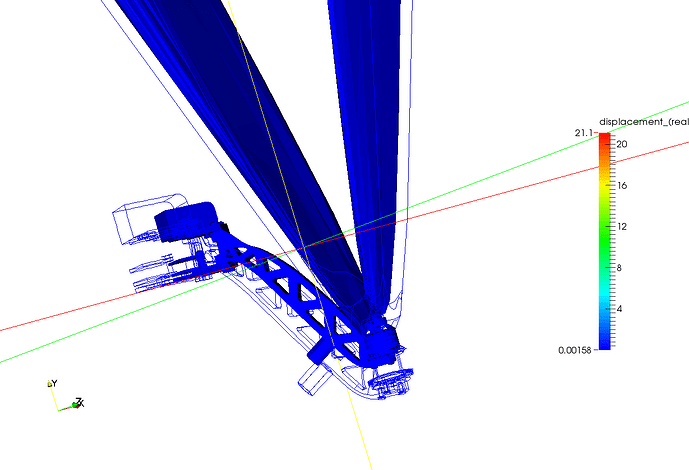
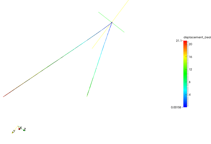
We will now investigate how the drone reacts to external periodic in the near of relevant eigenfrequencies.
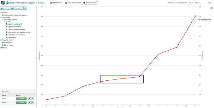
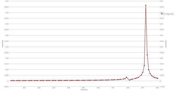
Taking a look at the result of our Level 1 homework will help to identify this eigenfrequencies. Since our engine is operating between 14000 and 20000 rpm which is equal to a frequency of 233 / 330 Hz we will only investigate the physical behavior of the drone for eigenmodes 5,6 and 7.
In Addition to that we will also investigate the effect of damping. All in all you will create six different runs for this level.
<img src=“/forum/uploads/default/original/1X/78989c06a72edb2acf4f95e0490030aa5f74b007.png” width=“690” height=“207”
Step-by-Step Instructions
Meshing
Since we will use the same geometry for the harmonic simulation it is not necessary to create a new mesh. We will just use the mesh from the previous Level 1 exercise.
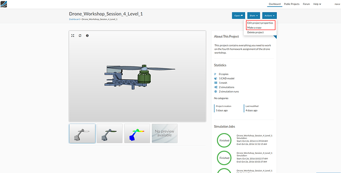
Now we will copy and rename the project to have an better overview. Therefore, copy and rename the project to ‘Drone_Workshop_Session_4_Level_2’ by first clicking on Make a copy, then Edit project properties under Actions and changing the project name.
Simulation Setup
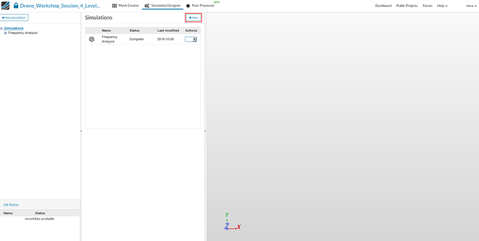
- Click on the Simulation Designer button in the main ribbon bar and then on New button.
This will open an additional column in the middle. Here you can select the type of simulation you want to run.
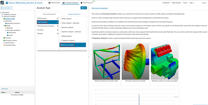
In our case we will run a Harmonic analysis simulation.
Next you have to specify which mesh you want to use for your simulation.
Domain
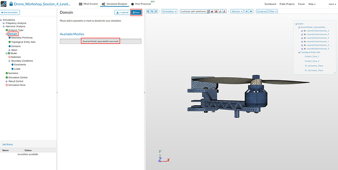
- Click on the Domain item in the project tree and select QuarterModel_separatedScrews mesh from the menu which disappears in the middle column. Don’t forget to Save your selection.
SimScale keeps all Topological Entity Sets which were assigned to a mesh. We can therefore use the as they are.
Contacts
Since we are simulating an assembly of two parts it is necessary to define Contacts which are describing the kinematic behaviour of the parts.
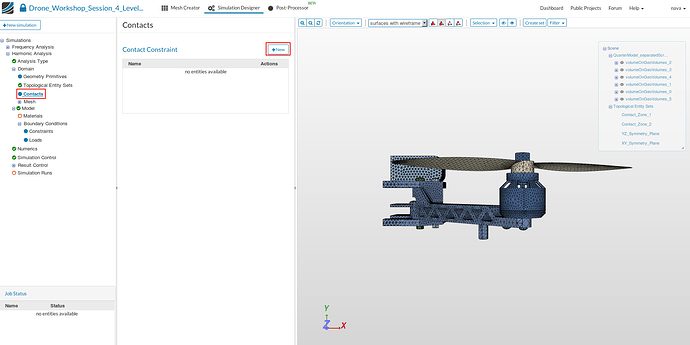
- Click on the Contacts item in the project tree which will open a new middle column menu where you can add new contacts by clicking on the New button.
Similar to Level 1 of this homework we will define all kinematic dependencies in one contact.
Contact
In this contact we will fix the assembly made of the battery, the frame, the screws, the engine and the propeller. Instead of selecting the faces for master and slave entity from the list or graphically we will use the face sets we created some minutes ago.
- Click on the Contacts item in the project tree which will open a new middle column menu where you can add new contacts by clicking on the New button.
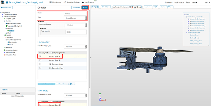
- Specify the following parameters:
- Name: Contact
- Type: Bonded Contact
- Master entity: Contact_Zone_1
- Slave entity: Contact_Zone_2
- Finally Save the settings.
Materials
Now we define and assign material properties to the different parts.
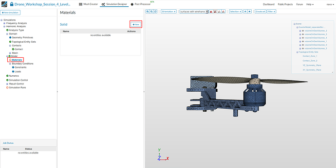
- Click on the Material item in the project tree. This will open a middle column menu where you can edit and create materials and assign them to volumes. Click on the New button
Now you can define your new material based on your own material properties or access our Material Library which includes ready-to-use material models for several materials.
We will start with the manual definition of materials:
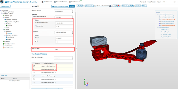
ABS Thermoplastics
- Specify the following parameters:
- Name: ABS Thermoplastic
- Young’s Modulus [N/m2]: 1800000000
- Poisson’s ratio: 0.35
- Damping: Rayleigh Damping
- αK [1/s]: 0.000037
- βM [s]: 1.5
- Density [kg/m3]: 1040
- Assign it to the drone body and the propeller (volumeOnGeoVolumes_4, volumeOnGeoVolumes_5) and finally Save the settings.
Add an additional material to your project tree.
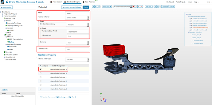
Battery
- Specify the following parameters:
- Name: Battery
- Young’s Modulus [N/m2]: 70000000000
- Poisson’s ratio: 0.34
- Damping: none
- Density [kg/m3]: 2500
- Assign the material to the battery of the drone (volumeOnGeoVolumes_0)and finally Save the settings.
Steel
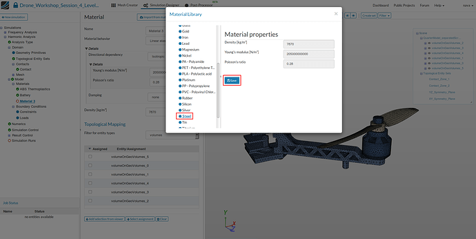
Next we will assign the steel material model to the screws and the engine. Add an additional material to your project tree.
Now we will access our material library instead of creating the material model manually.
- Click on the Import from material library which will open a widget.
- Please select steel from the list on the left side and save your selection by clicking the related button.
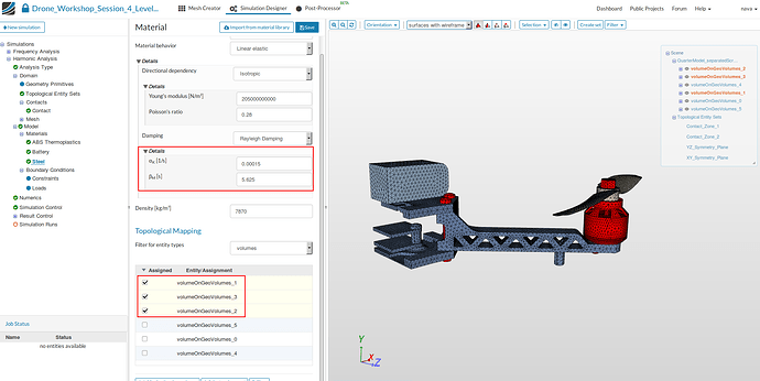
Change the damping properties:
- Damping: Rayleigh Damping
- αK [1/s]: 0.00015
- βM [s]: 5.625
- Now assign the material to the screws and the engine (volumeOnGeoVolumes_1, volumeOnGeoVolumes_2, volumeOnGeoVolumes_3).
Boundary Conditions
Next we can start to define the boundary conditions.
There are two kinds of boundary conditions for structural simulations.
- Constraint conditions are used to limit the degrees of freedom of the model.
- Load conditions are applying an external load to the model
We first add the constraint boundary conditions:
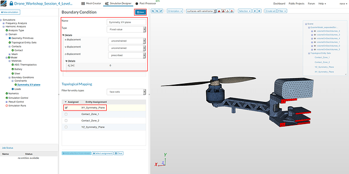
Symmetry XY-plane
This boundary condition is required because we are using a quarter model of the drone.
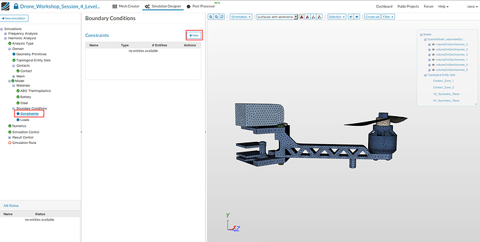
- Create a new constraint boundary condition by first clicking on the Constraint and then on New button.
- Specify the following parameters:
- Name: Symmetry XY-plane
- Type: Fixed Value
- x displacement: unconstrained
- y displacement: unconstrained
- z displacement: prescribed with a value of 0
- Finally, assign the boundary condition to the face set XY_Symmetry_Plane and then Save.
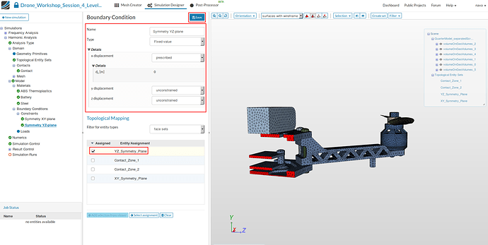
Symmetry YZ-plane
This boundary condition is required because we are using a quarter model of the drone.
- Create a new constraint boundary condition same as above.
- Specify the following parameters:
- Name: Symmetry YZ-plane
- Type: Fixed Value
- x displacement: prescribed with a value of 0
- y displacement: unconstrained
- z displacement: unconstrained
- Finally, assign the boundary condition to the face set YZ_Symmetry_Plane and then Save.
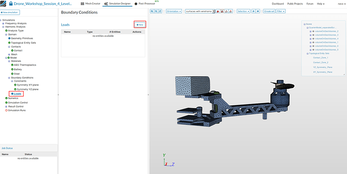
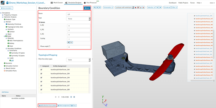
Now we will create a load boundary condition to apply the lift force.
- Create a new load boundary condition by clicking the related button.
- Specify the following parameters:
- Name: Lift (optional)
- Type: Force
- fx [N] : 0
- fy [N]: 2
- fz [N]: 0
- Scaling: 1
- Finally, assign the boundary condition to all faces of the blade of the propeller and Save.
- List of faces to select:
faceGroupOnGeoFaces_245, faceGroupOnGeoFaces_246, faceGroupOnGeoFaces_247, faceGroupOnGeoFaces_248, faceGroupOnGeoFaces_249, faceGroupOnGeoFaces_250, faceGroupOnGeoFaces_251, faceGroupOnGeoFaces_252, faceGroupOnGeoFaces_253, faceGroupOnGeoFaces_254, faceGroupOnGeoFaces_255, faceGroupOnGeoFaces_256, faceGroupOnGeoFaces_257, faceGroupOnGeoFaces_260, faceGroupOnGeoFaces_261, faceGroupOnGeoFaces_262, faceGroupOnGeoFaces_263, faceGroupOnGeoFaces_264, faceGroupOnGeoFaces_265, faceGroupOnGeoFaces_266, faceGroupOnGeoFaces_267, faceGroupOnGeoFaces_268, faceGroupOnGeoFaces_269, faceGroupOnGeoFaces_270, faceGroupOnGeoFaces_271, faceGroupOnGeoFaces_272
Simulation Control and Numerics
Numerics, which is the next item in the project tree, can be skipped since the default settings are fine.
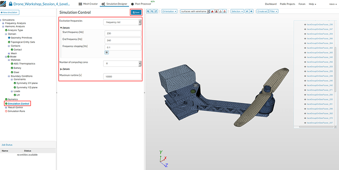
- Click on the Simulation Control item in the project tree to specify the last details of your simulation.
- Excitation frequencies: frequency list
- Start frequency [Hz]: 230
- End frequency [Hz]: 240
- Frequency stepping [Hz]: 0.1
- Number of computing cores: 8
- Maximum runtime [s]: 10000
Result Control
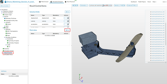
Finally we will add some Point data items to simply the result interpretation.
- Click on the Result Control item in the project tree which will open a new middle column menu.
- Click on the New button in the middle column menu will create a new Point data item.
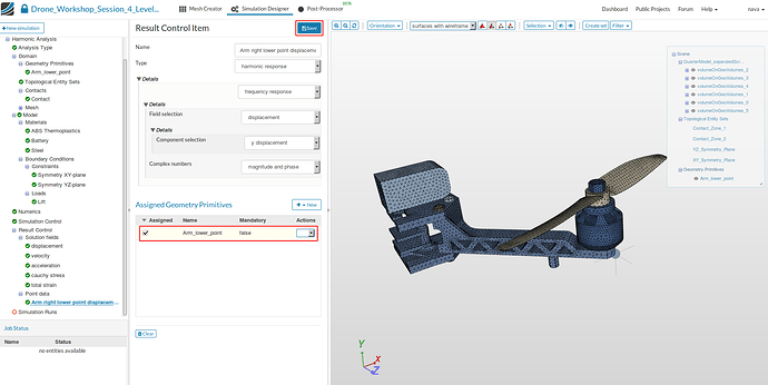
Arm right lower point displacement
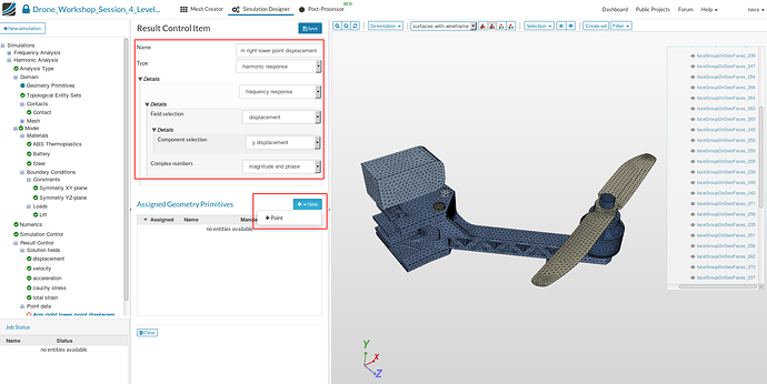
- Specify the following parameters:
- Name: Arm right lower point displacement (optional)
- Type: harmonic response
- Frequency response
- Field selection: displacement
- Component selection: y displacement
- Complex numbers: magnitude and phase
Now we have to create a Geometry Primitive since this analysis type does not support to select points or nodes directly.
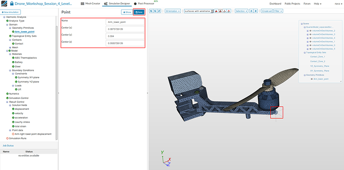
-
Click on New and then on Point which will open a new middle column windows where you can define the primitive, as shown in the figure above.
-
Specify the following parameters:
- Name: Arm_lower_point (optional)
- Center (x): 0.0875726139
- Center (y): 0.004
- Center(z): 0.0930726139
- Save the point by clicking on Save button.
Now switch back to the Point data item you created and map it to the primitive.
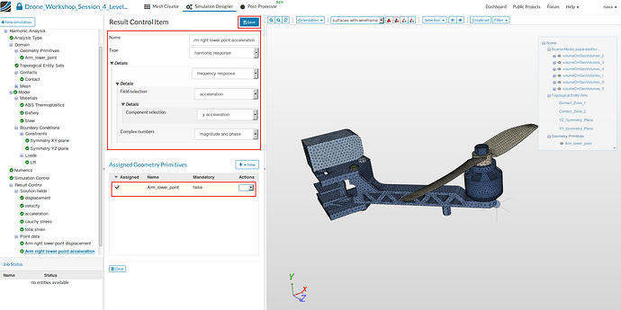
Arm right lower point acceleration
- Specify the following parameters:
- Name: Arm right lower point displacement (optional)
- Type: harmonic response
- Frequency response
- Field selection: acceleration
- Component selection: y displacement
- Complex numbers: magnitude and phase
- Map this item again on the primitive and Save the settings.
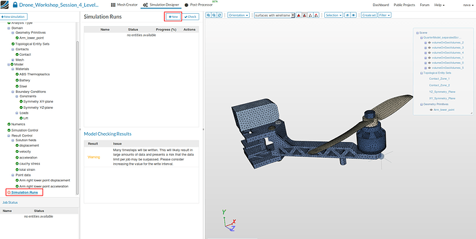
Simulation Runs
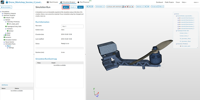
- To start the simulation, click on the Simulation Runs item in the tree and click on the New button at the top of the middle column menu. This will create a snapshot of your simulation settings as a new sub-item.
- You can now start the simulation run by selecting it from the project tree and then click on the Start button.
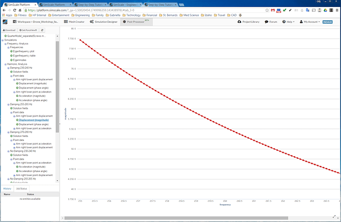
Once your simulation is finished you can do the post processing using the workflows you already know from the last homework assignments.
Important note
It is not necessary to set up the simulation from scratch in order to simulate the five other setups. You can just modify your simulation and create a new run. Make sure to update the following settings.
- To simulate the three runs without damping you have to change the related entry in the material models for ABS Thermoplastic and Steel (Damping: none)
- Use following Simulation Control settings for the other two eigenfrequencies:
- (Start frequency: 255, End frequency: 265, Frequency stepping: 0.1)
- (Start frequency: 270, End frequency: 280, Frequency stepping: 0.1)
Congratulations, you have completed the Homework of Session 4 - Level 2 and can now move on to Session 5:
