Aerodynamics of Perrinn LMP1: Investigating the drafting and overtaking conditions as well as driving in a Yaw angle

[roozbehmousavi]

The present project is aimed to investigate the aerodynamics of an LMP1 racing car designed by the Nikolas Perrinn’s team. In addition to the aerodynamics of a single car, the drafting and overtaking characteristics of the car is investigated. Moreover, the aerodynamic performance of the car in a non-zero Yaw angle is investigated. Some quantitative information on the flow and geometrical conditions are as follows:

• The speed of the car is set to 250 km/h.

• In the case of the drafting cars, the distance between the front of the car that drives ahead and the front of the other car is 5.5m. It means that the cars drive with a distance of around 0.85m.

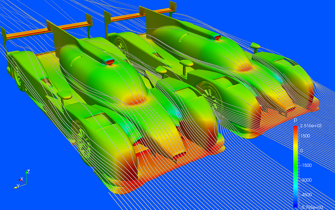
• In the case of the overtaking cars, the distance between the cars is 0.25m.

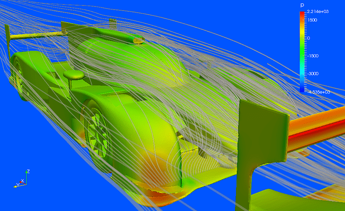
• For the case with a non-zero Yaw angle, the Yaw angle is set to 10 degrees.

A link to the project: Perrin-LMP1 by roozbehmousavi | SimScale

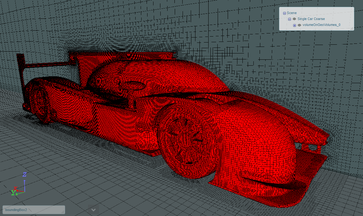
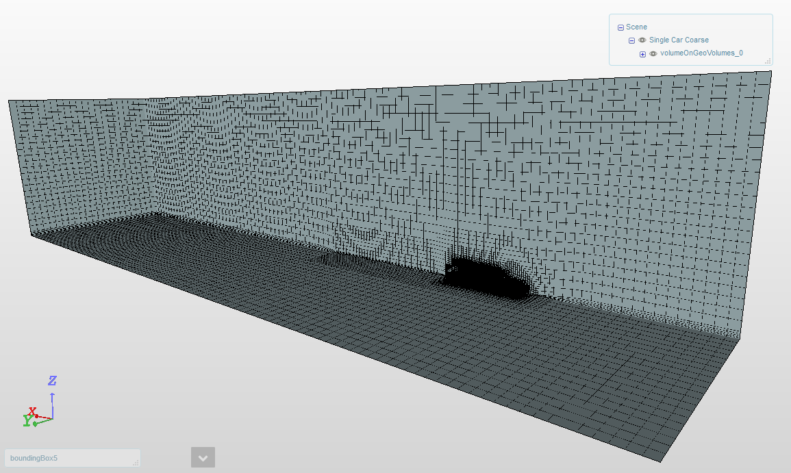
The following picture shows the grid used for a single car.

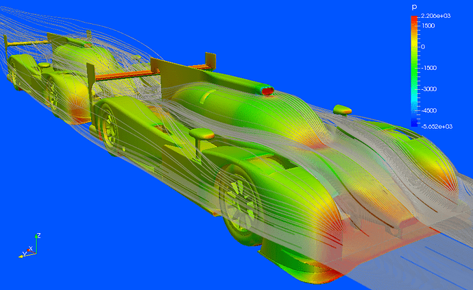
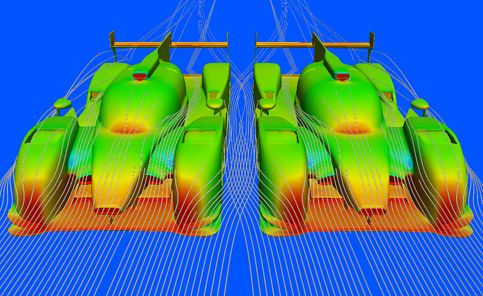
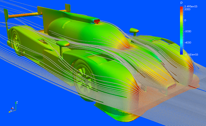
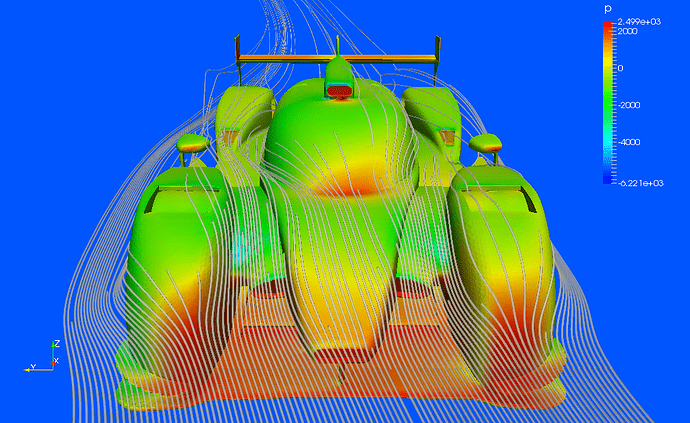
The following pictures show the pressure field over the surface of the car for different cases, as well as the streamlines:

• Single car
  

  

• Drafting cars
  

  

• Overtaking cars
  
  

• Single car in a Yaw angle
  
  

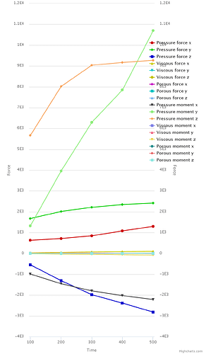
The drag force (D), the lateral force (B) and the vertical force (L) exerted on the cars in different cases, are as follow:

• Single car:
  D = 1199.42N
  B = 0
  L = -3182.23N

• Drafting cars:
  Note: As a result of the high resolution of the STL file, the file could not be opened in my CAD software as a solid body. Therefore, I had to use the software meshLab to make a system of two cars. But the both cars could only be exported as a single surface. Consequently, the forces are computed for the both cars:
  D = 1398.97N
  B = 0
  L = -2808,10N

• Overtaking cars:
  D = 2541.14N
  B = -621.17N
  L = -7285.12N

• Single car in Yaw:
  D = 2392.72N
  B = 2731.24N
  L = -6504.74N

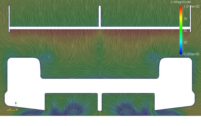
As it is shown in the pictures, in the case of the drafting cars, the streamlines are less curved toward the car that drives behind. This explains a reduction of the downforce exerted on that car.

In the case of the overtaking cars, as it is shown in the second pictures, the streamlines of each car in the space between the cars, are deviated toward the other car. This explains the lateral force exerted on each of the cars toward the other car.

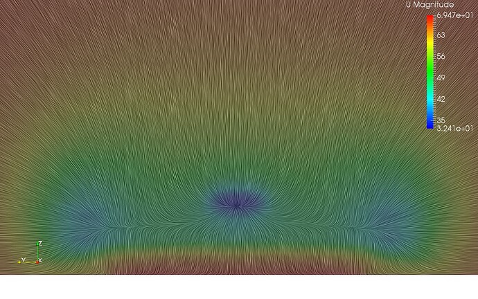
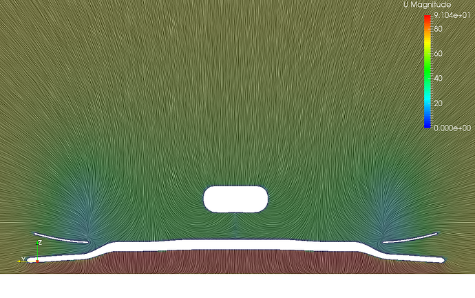
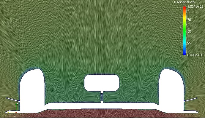
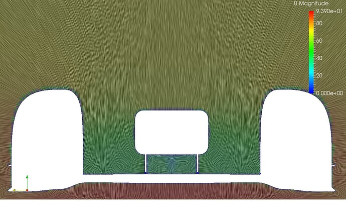
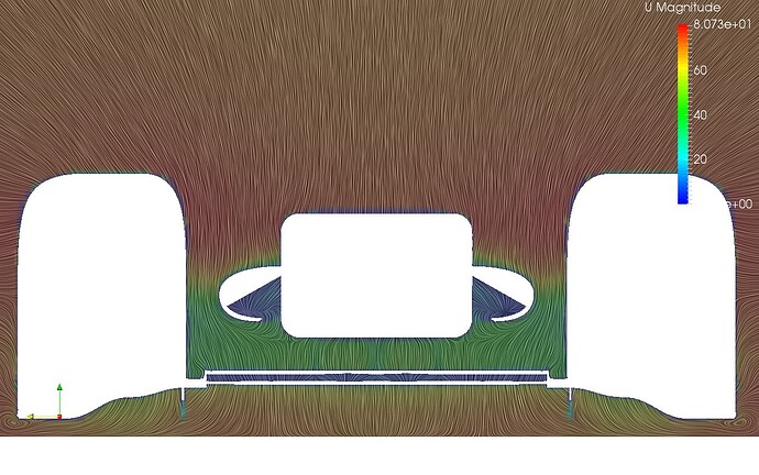
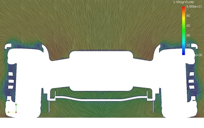
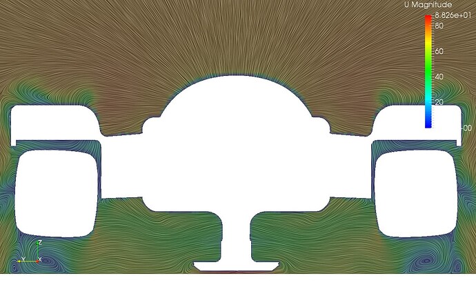
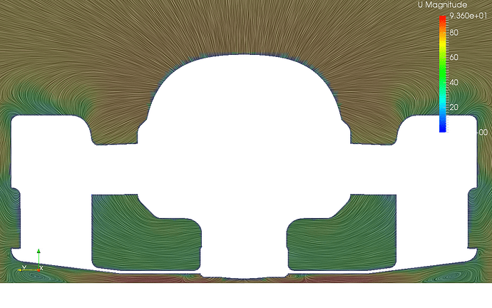
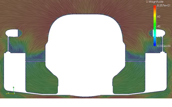
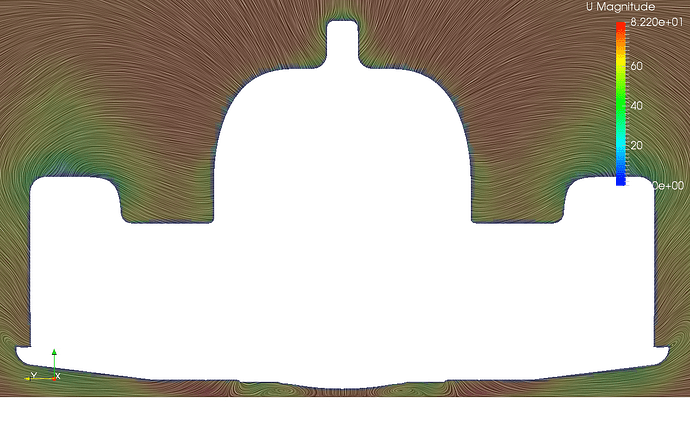
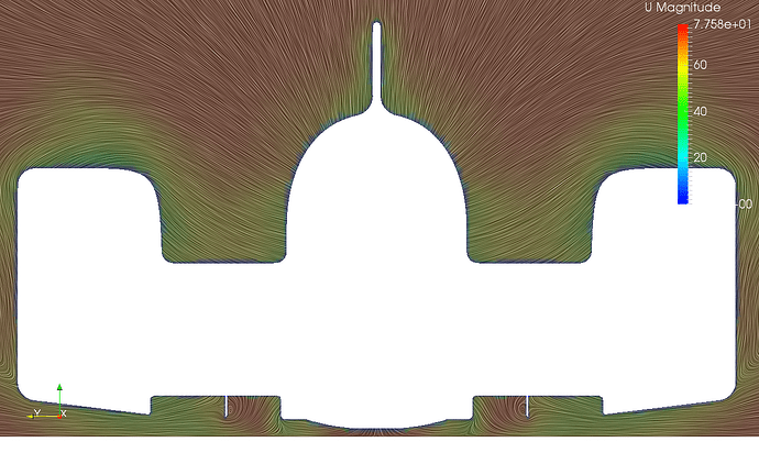
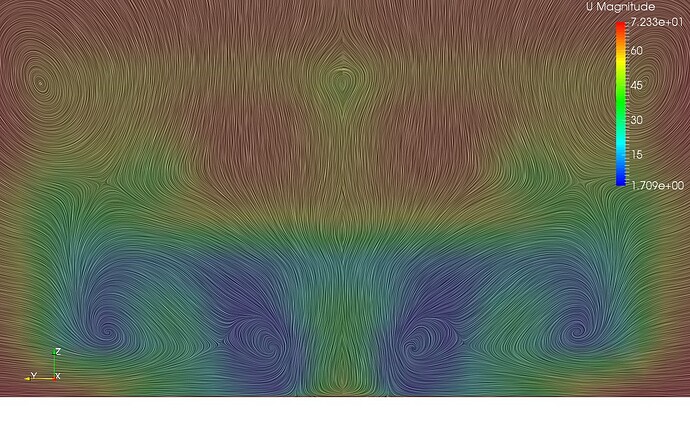
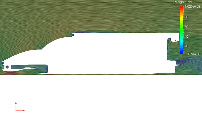
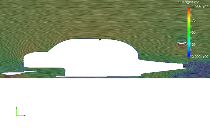
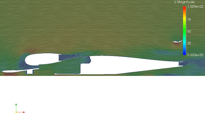
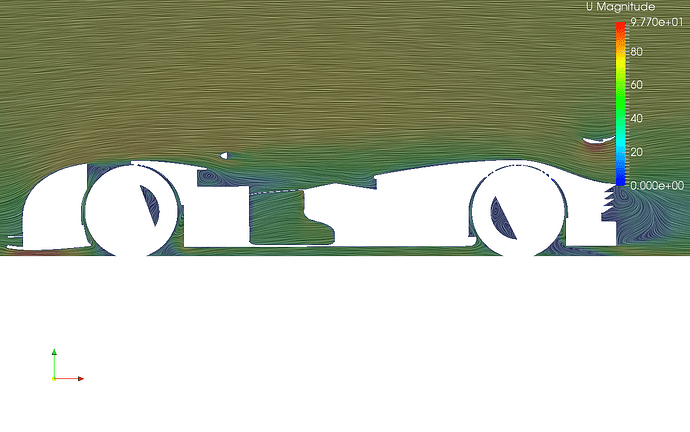
The following pictures show the flow field around the single car in different streamwise and lateral sections. (The x-coordinate of the front of the car is -1 and y-coordinate of the centroid of the car is 0)
x = -1m

x = -0.9m

x = -0.8m

x = -0.6m

x = -0.4m

x = -0.1m

x = 0.3m

x = 0.5m

x = 0.75m

x = 2m

x = 2.5m

x = 3m

x = 3.5m

x = 4m

x = 5m

y = 0m

y = 0.25m

y = 0.5m

y = 0.75m

[roozbehmousavi]

Hi everyone, I need to correct something in the report. The forces which are calculated for the Single car as well as the drafting cars, are for the half of the bodies. So, you need to double these values. Sorry for the inconvenience!

(@AnnaFless )

[roozbehmousavi]

A nice review article:

Ground Effect Aerodynamics of Race Cars

[AnnaFless]

@roozbehmousavi, got it. Thanks for posting the correction!

[Milad_Mafi]

This is awesome! Great work!

I have two suggestions which could help to improve the accuracy of your results

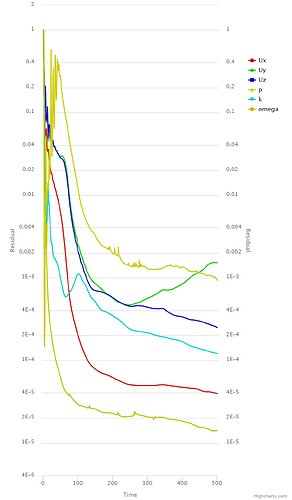
• First of all it seems that your simulation is not fully converged. As an example you should take a look at the simulation of “Drafting Cars”. Especially the forcs are not converged already. I would suggest to run additon 1000 iterations.
  
  

• Using layer elements will help to resolve transition and boundary layer effects

Cheers,

Milad

[roozbehmousavi]

Hi @Milad_Mafi ,
Many thanks for your comments. You are right, the solution for this case needs more iterations. Concerning the grid generations, I had some strange difficulties which were somehow related to the *.stl CAD file, I guess. First of all, I could not extract the edges using a feature angle criterion. I also could not open the file as a solid body in SolidWorks because of the high resolution and I had to use MeshLab to make two drafting cars. But the problem was that the two cars were exported as a single surface. This prevented to make a surface refinement! It would be great if I could have a *.step file of this geometry.
You are absolutely right about the boundary layer mesh. Honestly I did not try that with the coarse grid, but it did not work for the fine grid. I got errors. The bounday layer mesh is very necessary for capturing the separation zone precisely, but there is nothing to do with the transition, in my opinion. For capturing the transition line, one has to use either LES or a transitional RANS model solving a turbulence intermittency equation.
I should also say that I had some stability problems during the flow simulation using the fine grid. If you look at the grid (https://www.simscale.com/workbench/?pid=1992874712637604373#tab_0-0), you will find it quite nice and you see that all the details of the geometry (for example the space between the wheel and the body of the car) are precisely resolved. I have no idea what is the origin of the solution instability concerning this fine grid.

Regards,
Roozbeh

[dheiny]

@roozbehmousavi - awesome post-processing! Great project!

[roozbehmousavi]

(@dheiny ): Thanks Mr. Heiny!

[dylan]

I am interested if you can elaborate. It is impossible to diagnose without knowing what instability it is.

[roozbehmousavi]

Hi @dylan , thanks for your interest. It would be great if you try with the fine mesh and let me know about your experience. The fine grid looks OK, but the simulation is stopped at the first iteration. I tried to use lower relaxation factors, but with no successes. It seems that the problem is somehow related to the pressure solver that can not manage to handle such a huge spars matrix. I am looking forward to hear good news from your simulation.

[dylan]

The fine mesh won’t run because it has failed checkMesh:

Checking geometry...
    Overall domain bounding box (-11 -0.000530918 -0.0375) (39 11 11)
    Mesh (non-empty, non-wedge) directions (1 1 1)
    Mesh (non-empty) directions (1 1 1)
    Boundary openness (-3.61347e-16 5.91293e-15 -2.25693e-15) OK.
 ***High aspect ratio cells found, Max aspect ratio: 1.82536e+195, number of cells 10
  <<Writing 10 cells with high aspect ratio to set highAspectRatioCells
    Minimum face area = 3.95633e-09. Maximum face area = 0.071144.  Face area magnitudes OK.
 ***Zero or negative cell volume detected.  Minimum negative volume: -9.07755e-09, Number of negative volume cells: 10
  <<Writing 10 zero volume cells to set zeroVolumeCells
    Mesh non-orthogonality Max: 175.416 average: 8.48142
   *Number of severely non-orthogonal (> 70 degrees) faces: 37.
 ***Number of non-orthogonality errors: 15.
  <<Writing 52 non-orthogonal faces to set nonOrthoFaces
 ***Error in face pyramids: 74 faces are incorrectly oriented.
  <<Writing 66 faces with incorrect orientation to set wrongOrientedFaces
 ***Max skewness = 104.595, 368 highly skew faces detected which may impair the quality of the results
  <<Writing 368 skew faces to set skewFaces
    Coupled point location match (average 0) OK.

Failed 5 mesh checks.

The more the stars, the worse the problem. But it is I believe the negative cell volumes that kill the job.
The coarse mesh ran because checkMesh only returned:

Checking geometry...
    Overall domain bounding box (-11 -0.000567249 -0.0375) (39 11 11)
    Mesh (non-empty, non-wedge) directions (1 1 1)
    Mesh (non-empty) directions (1 1 1)
    Boundary openness (-6.24213e-17 3.15063e-16 1.35568e-15) OK.
    Max cell openness = 4.33442e-16 OK.
    Max aspect ratio = 38.3736 OK.
    Minimum face area = 1.5103e-07. Maximum face area = 0.273126.  Face area magnitudes OK.
    Min volume = 6.08063e-09. Max volume = 0.132627.  Total volume = 6068.62.  Cell volumes OK.
    Mesh non-orthogonality Max: 64.977 average: 8.98473
    Non-orthogonality check OK.
 ***Error in face pyramids: 1 faces are incorrectly oriented.
  <<Writing 1 faces with incorrect orientation to set wrongOrientedFaces
 ***Max skewness = 15.2136, 131 highly skew faces detected which may impair the quality of the results
  <<Writing 131 skew faces to set skewFaces
    Coupled point location match (average 0) OK.

Failed 2 mesh checks.

High skewness may or may not affect convergence/accuracy depending where the cells are located. If they are in regions with low gradients they are fine. There is only one wrongly oriented cell, which may also be located somewhere with low field gradients; maybe that’s why the case converged.

[dheiny]

@dylan - good catch. Negative volume cells are indeed a show-stopper for the sim.

[dylan]

Now, lets talk about meshing with cut cells. For a complicated geometry like a racing car, you would want to split the stl file into multiple files and apply name-based local refinement. This way you obtain not only a better control over local cell sizes, but also a better capture of important edges as now patches/subsets along with their shared boundaries are recognised by the mesh generator. Finally, it is much easier to grow boundary layer cells on a good surface mesh.

Currently, surface split is easily done in native OpenFOAM with a collection of its utilities for surface mesh manipulation. I haven’t noticed such functions on the SimScale platform with a community plan.

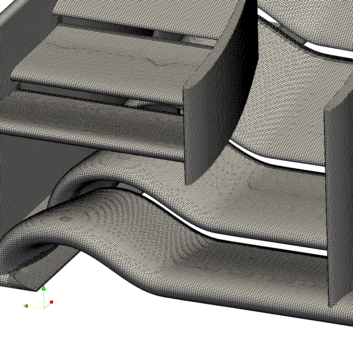
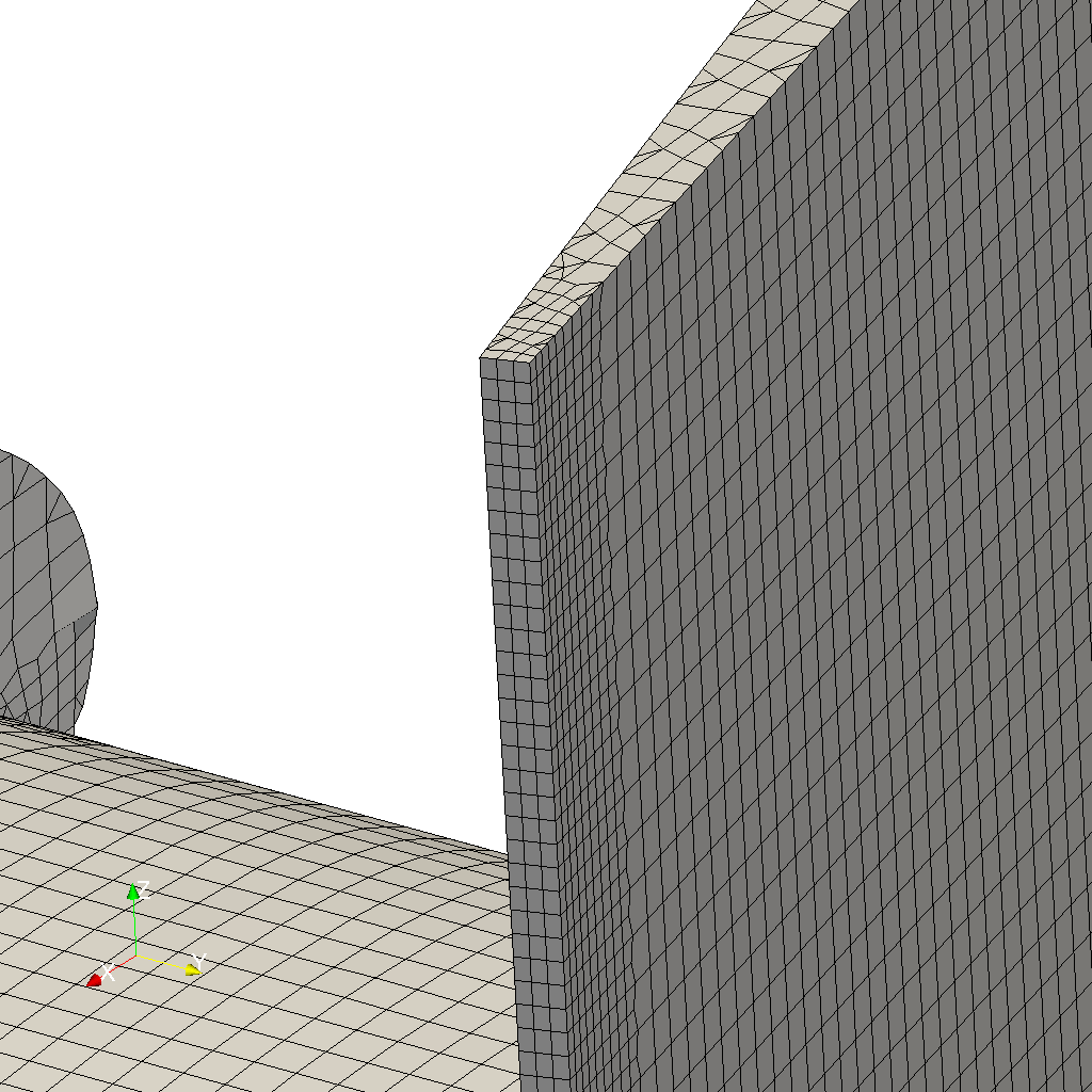
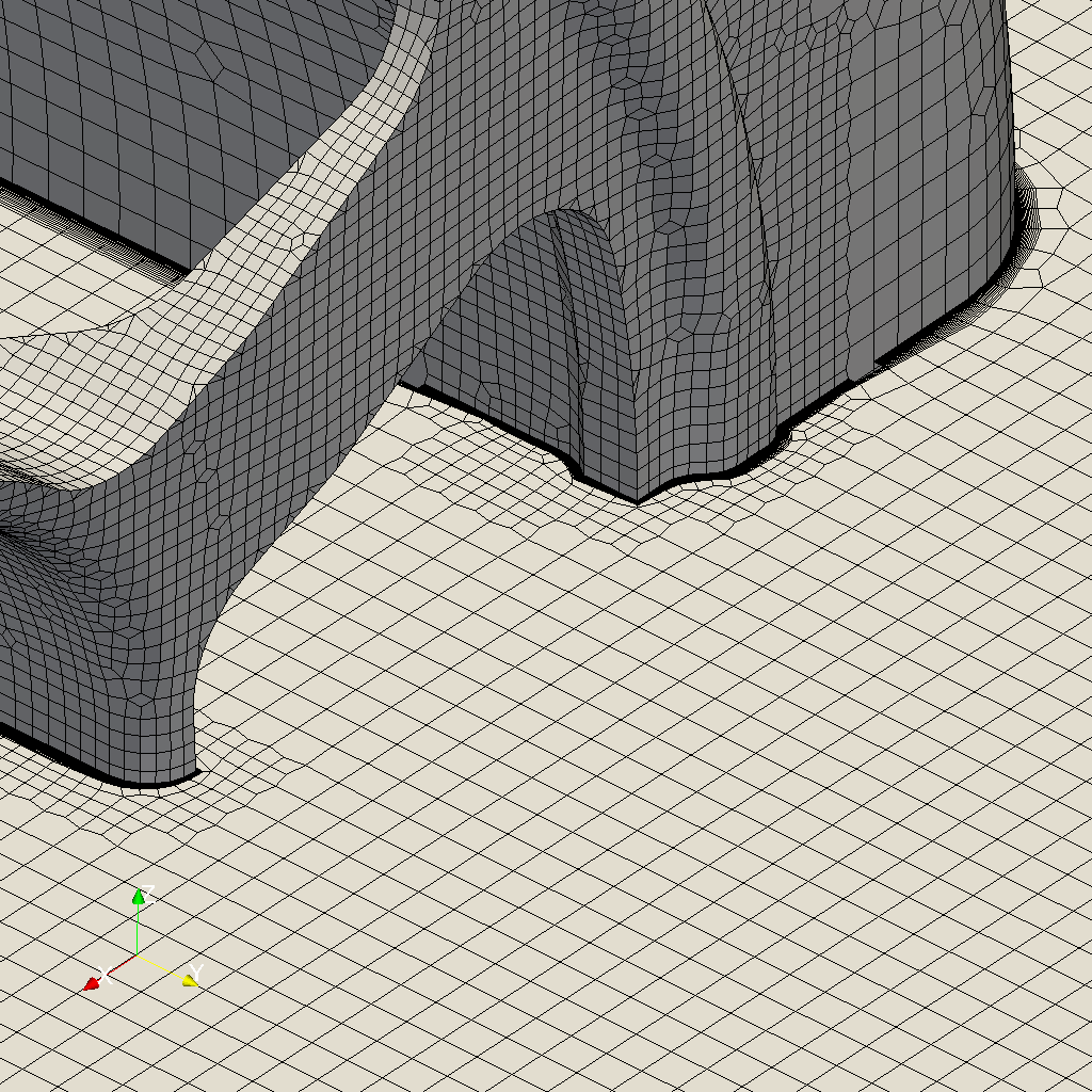
I have meshed multiple automotive/motorsport parts with structure/unstructured cells and am currently doing a PhD on aeroacoustics. I have found it very handy to let CAD do the hard work, although for relatively small/simple motorsport parts, splitting an stl file in native OpenFOAM can save me some time. An example of the F1 front wing from an early workshop SimScale organised is provided below:

whose checkMesh returns:

Checking geometry...
    Overall domain bounding box (-4.5 -3.88524e-08 0) (8.5 2.5 2.76)
    Mesh (non-empty, non-wedge) directions (1 1 1)
    Mesh (non-empty) directions (1 1 1)
    Boundary openness (-8.18583e-18 -1.60872e-16 -4.17722e-17) OK.
    Max cell openness = 4.00464e-16 OK.
    Max aspect ratio = 11.5065 OK.
    Minimum face area = 1.19661e-11. Maximum face area = 0.917718.  Face area magnitudes OK.
    Min volume = 3.38159e-13. Max volume = 0.743455.  Total volume = 89.6918.  Cell volumes OK.
    Mesh non-orthogonality Max: 71.5482 average: 6.0495
   *Number of severely non-orthogonal (> 70 degrees) faces: 2.
    Non-orthogonality check OK.
  <<Writing 2 non-orthogonal faces to set nonOrthoFaces
    Face pyramids OK.
    Max skewness = 3.68145 OK.
    Coupled point location match (average 0) OK.

Mesh OK.

One doesn’t worry too much about non-orthogonality, as corrections can be applied in solvers.

Note that no boundary layers have been added, because a set of closely controlled/monitored cell optimisation parameters is required to smooth out those cells. But the main reason it is not done on this particular wing is because there are 800k surface cells, on which if 20 boundary layers are grown, my laptop will not have enough RAM to even visualise the volume mesh ( need at least 10G of RAM to load it ).

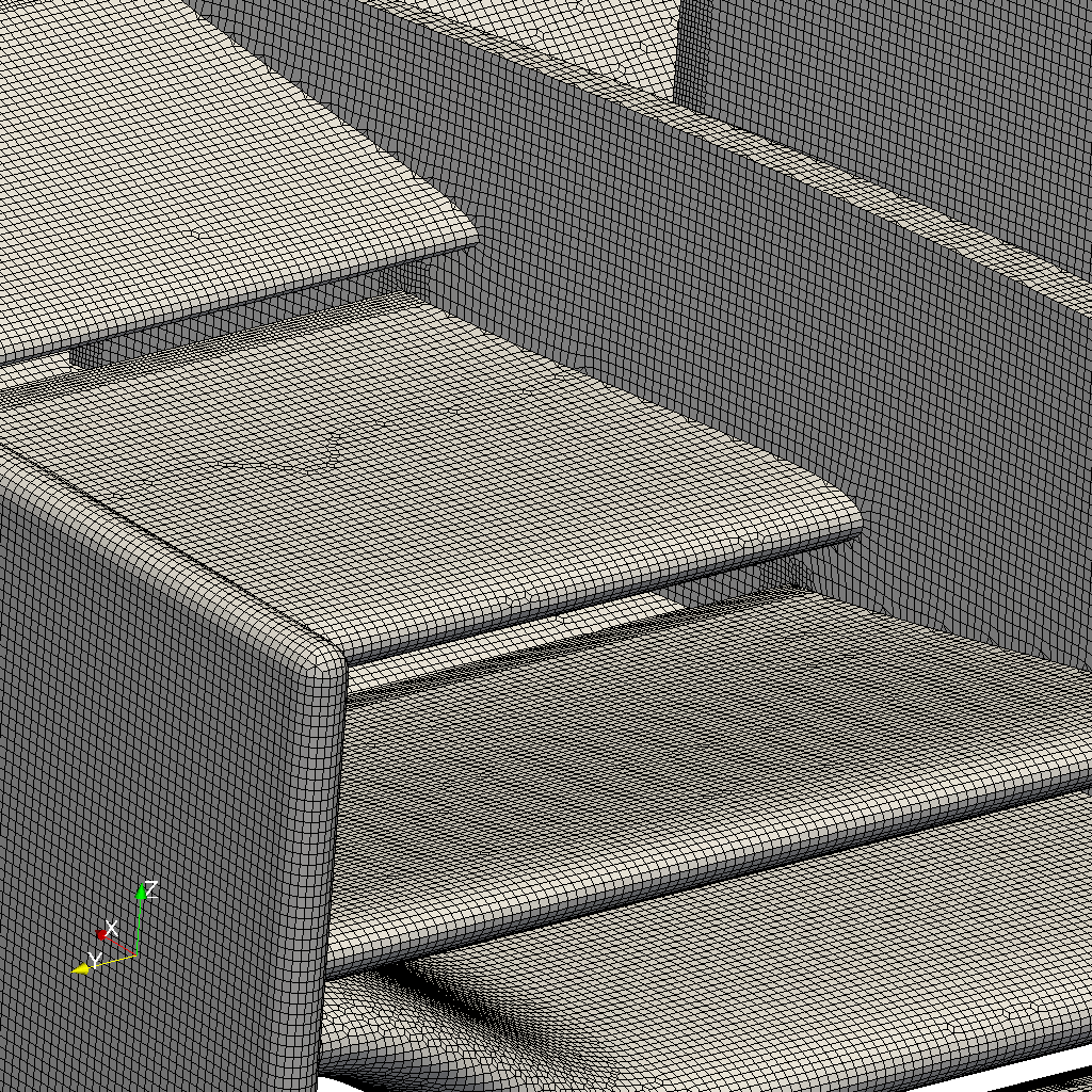
But I do have a smaller mesh ( a wheel ) in which 20 boundary layers were added:

whose checkMesh returns:

Checking geometry...
    Overall domain bounding box (-10 0 0.389722) (40 6 8.4)
    Mesh (non-empty, non-wedge) directions (1 1 1)
    Mesh (non-empty) directions (1 1 1)
    Boundary openness (3.78916e-19 3.78831e-16 -4.22083e-16) OK.
    Max cell openness = 3.48028e-15 OK.
    Max aspect ratio = 127.821 OK.
    Minimum face area = 1.01365e-09. Maximum face area = 1.1977.  Face area magnitudes OK.
    Min volume = 3.18048e-12. Max volume = 1.33059.  Total volume = 2399.94.  Cell volumes OK.
    Mesh non-orthogonality Max: 73.3458 average: 7.22503
   *Number of severely non-orthogonal (> 70 degrees) faces: 100.
    Non-orthogonality check OK.
  <<Writing 100 non-orthogonal faces to set nonOrthoFaces
    Face pyramids OK.
    Max skewness = 2.90826 OK.
    Coupled point location match (average 0) OK.

Mesh OK.

As you can see, a set of clean stl files give you a good surface mesh and from there you may obtain a good boundary layer too.

[dylan]

I just spot another problem with the coarse mesh run. The absolute tolerance for the velocity fields are not small enough and Ux is no longer solved for the last few iterations:

Time = 500
DILUPBiCG: Solving for Ux, Initial residual = 6.50226222661e-06, Final residual = 6.50226222661e-06, No Iterations 0
DILUPBiCG: Solving for Uy, Initial residual = 1.93712216115e-05, Final residual = 4.70660878179e-06, No Iterations 1
DILUPBiCG: Solving for Uz, Initial residual = 1.37544730886e-05, Final residual = 8.88866037304e-06, No Iterations 1
GAMG: Solving for p, Initial residual = 4.4842154963e-05, Final residual = 8.93812980345e-07, No Iterations 4
GAMG: Solving for p, Initial residual = 4.94288599942e-06, Final residual = 8.29047562769e-07, No Iterations 1
GAMG: Solving for p, Initial residual = 1.09243422113e-06, Final residual = 5.23396505342e-07, No Iterations 1
time step continuity errors : sum local = 9.79919233392e-07, global = 2.4500148777e-08, cumulative = -0.00196944950993
DILUPBiCG: Solving for omega, Initial residual = 9.4735963376e-06, Final residual = 9.4735963376e-06, No Iterations 0
DILUPBiCG: Solving for k, Initial residual = 9.80221724403e-06, Final residual = 9.80221724403e-06, No Iterations 0
ExecutionTime = 1006.11 s ClockTime = 1014 s

The turbulence parameters k and omega are not either.
A reduced tolerance is desired.

[dheiny]

@dylan - awesome images, thanks for sharing. What tools did you use for the actual meshing? snappy? A couple of points:

• There is no difference in the feature set for community and professional plan, so everybody has access to all simulation features here on SimScale
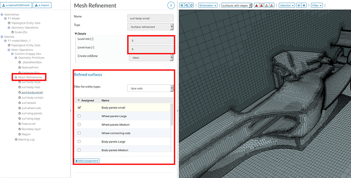
• Local refinements based on specific surfaces is possible with SimScale, check out the screenshot below. You can address all surfaces of a model with a desired refinement level and also add region/primitive based refinements

• “Splitting of geometry”: Generally the SimScale workflow is designed open, which means whatever you prefer doing locally / with your own tools you should be able to do it locally. So you could do splitting locally and then upload the splitted STL - SimScale will recognize each surface and you can assign mesh refinements onto them

• Working with NURBS models: Agreed - let the CAD system do, what it can do best. So if you’re working in a BREP modeler, you can also upload the STEP model such that SimScale will take care of the tessellation if necessary.

Hope that helps.

[dheiny]

@dylan - forgot to mention: keep the feedback coming, we’re eager to improve the workflow!

[dylan]

Hi,

Thank you for those images. I didn’t notice those features.

Now about my unstructured meshes. I am using both SnappyHex and cfMesh, the latter being another open-source mesh generator for OpenFOAM. The wing was created in SnappyHex and the wheel with boundary layers cfMesh. They both provide cut cells and are easy to implement. However, cfMesh has been a lot faster and more efficient for me despite less control entries in its mesh dictionary. SnappyHex allows for more parameter tuning in the mesh dictionary and some of those features are very useful in complicated cases.

Sorry the images of the wing were also from cfMesh, but I do have the same wing meshed by SnappyHex and was equally good.

[dylan]

Hi,

About the geometry split, a GUI environment is easy to be made a meshing Swiss knife. There are a brunch of STL manipulation utilities in OpenFOAM. One can use surfaceAutoPath name.stl newName.stl [angle] to split one large STL file into multiple parts within the same file. From there, executing surfaceSplitByPatch newName.stl will turn the one large file into multiple STL files, each containing one patch as split before. Now, with the GUI environment, one can go ahead and rename, delete, or combine those STL files. Finally, it is not hard and useful to combine all the patches into one STL file that contains all the individual names by using cat name* > newerName.stl.

Now, the amount of new patches generated by surfaceAutoPatch can range from 2 to 20000, depending on what angle is chosen and how clean the surface mesh is. With a dirty STL file, which is almost always the case, one will easily end up dealing with a few thousands of STL patches. This is where a GUI environment is highly appreciated, as it allows visual/manual interactions.

The above is only a small section of the surface mesh utilities that come with the OpenFOAM release but can potentially provide significant improvement in meshing efficiency, and reduced CAD usage.

The wheel mesh I uploaded was purely done with the STL manipulation utilities mentioned above in a TUI environment/Paraview, as there are only a few patches/shared edges that need to be recognised by the mesh generator.

[dheiny]

@dylan - yes, these OpenFOAM manipulation utils are indeed neat. However most of the users here prefer to work with the actual NURBS model (e.g. STEP, IGES) where surface-splitting and merging is not relevant. By definition you can address the entire topology of those models, also during snappyHexMesh setup. But it seems that you prefer to work with the faceted model. Is there a specific reason for this? Do you want to have full control over the surface tessellation?

[dylan]

Hi,

I havent used stp/iges here and didn’t think I saw any public projects done that way. Could you please link me to one example as such? I would like to see how local refinements are applied when meshing with stp/iges.

There are two reasons I would like to split a geometry. Firstly, it is possible to capture all the important edges as all the patches and their shared boundaries are stored in the combined surface mesh file. Secondly, working with different patches is useful when saving computation power is desired as I gain full control over local cell size. If the same goals can be achieved with stp/iges through different meshing approaches, then why not.