This article shows a basic approach to set up an atmospheric boundary layer (ABL). We will go through the formulation and set up parameters answering the following questions:
- How can one set up an Atmospheric Boundary Layer (ABL) profile at the inlet?
- What formulas can be used for it?

Important
The concepts and workflow below can be applied to the fluid dynamic solvers based on OpenFOAM®.
Atmospheric Boundary Layer Overview
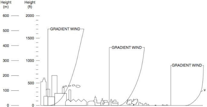
Generally speaking, an atmospheric boundary layer (ABL) consists of the lower regions of the atmosphere, which are still influenced by the earth’s features and processes. For CFD applications, we are mostly interested in the developed velocity and turbulence profiles.
In some fields, such as the architectural industry, setting a velocity profile at the inlet may be required. Prescribing an ABL can also be important in some applications, such as:
- Wind comfort analysis;
- External aerodynamics in general (cars, cities);
- Any other application where a developed velocity profile at the inlet is relevant.
Model For an ABL Profile
The presented model is based on [2]. There are different formulas available to model an ABL profile. The following abstract is presenting them:
Velocity
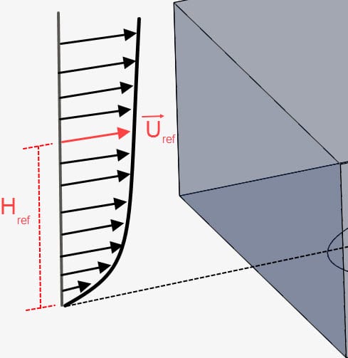
The velocity is a logarithmic profile, starting at 0 \(m/s\) on the ground. It’s, therefore, a function of height (z):
$$u(z) = \frac{u^{*}}{K} \cdot ln \left (\frac{z + z_{0}}{z_{0}} \right )$$
Where:
- K is the von Karman constant, usually taken in the range of 0.40 ± 0.02;
- z is the height in which the velocity is calculated;
- z0 is the aerodynamic roughness length. Still according to [2], the values for z0 vary based on landscape:
- 0.0002 for sea or lakes;
- 0.005 for smooth landscape, without obstacles/vegetation;
- 0.03 in case of an open land with grass;
- 0.1 for a cultivated area (farms, small obstacles);
- 0.25 if high crops and scattered obstacles are present;
- 0.5 for large vegetation, farms, clumps of forest;
- 1 for a closed landscape, like mature forests and homogeneous cities and villages;
- 2 or higher for centers of large towns, areas with buildings or forests with irregular height.
- u* is the friction velocity, given by:
$$u^{*} = K \cdot \frac{u_{ref}} {ln \left (\frac{H_{ref} + z_{0}} {z_{0}} \right )}$$
\(u_{ref}\) and \(H_{ref}\) are in Figure 2 below.

Turbulent Kinetic Energy (k)
Find the formula for the turbulent kinetic energy (k) below. \(c_\mu\) is the turbulent viscosity constant, equal to 0.09:
$$k(z) = \frac{{u^{*}}^{2}} {\sqrt{c_{\mu}}}$$
Turbulence Dissipation Rate (\(\epsilon\))
This equation is only necessary in case a k-epsilon turbulence model is being used:
$$\epsilon (z) = \frac{{u^{*}}^{3}} {K(z+z_0)}$$
Specific Dissipation Rate (\(\omega\))
k-omega and k-omega SST turbulence models require an input for \(\omega\):
$$\omega (z) = \frac{u^{*}}{K \sqrt{c_{\mu}}} \cdot \frac{1}{z + z_{0}}$$
Atmospheric Boundary Layer Setup
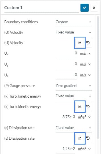
To input these formulas, one must create a custom boundary condition. After changing a parameter to a fixed value, it will be possible to use formulas as input. To access the formula input tab, click on the icons highlighted in the figure.
Check out this advanced tutorial if you are interested in a simulation using an ABL profile.
References
- Gaetani, I. Energy saving potential of night natural ventilation in the urban environment: the effect of wind shielding and solar shading. MSc thesis. Milan. 2013.
- BCA Green Mark for Residential Buildings: Technical Guide and Requirements. 2016. Available at https://www1.bca.gov.sg/docs/default-source/docs-corp-buildsg/sustainability/gm-rb-2016-technical-guide-_rev010120.pdf
Note
If none of the above suggestions solved your problem, then please post the issue on our forum or contact us.
