Thanks many times to you, @DaleKramer for your work on meshing and your direct help on this project. I was lost before and I didn’t know how much. Following the CFD master class, I naively expected that an incomplete boundary layer would simply change the magnitude of my results. In fact it completely changes the flow characteristics across a model, as I’ll show below. I was finding the results from my initial analysis really confusing and now I know why: I had a really crappy mesh with an overly-large boundary layer and poor coverage.
Side note: perhaps this is a trivial finding for you CFD experts out there, but for people like me (engineer with little experience in complex physics simulations), it’s super important. The accessibility of SimScale make it really tempting to throw something together and end up with a garbage-in/garbage-out result. I’ve seen more and more engineering candidates come through my door lately with an over-reliance on FEA/CFD methods and not enough skepticism or sophistication to even attempt corroborating the results with experiments or hand calcs. I’m hoping this post will serve as a warning for how wrong it can really be even if it looks right.
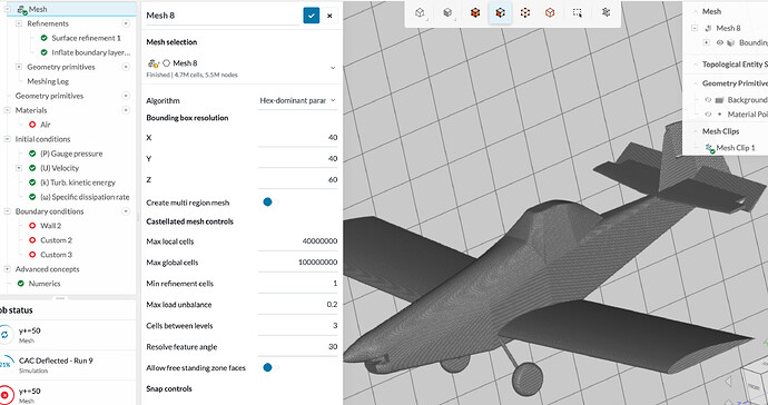
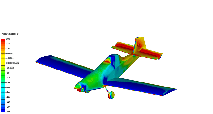
My original mesh, developed using the various refinements recommended in car/truck/plane tutorials and example projects I found in the Public Projects. I included surface refinements, boundary layer inflation, feature refinement, and some detailed flow volumes. Total cells: 6.8MM.
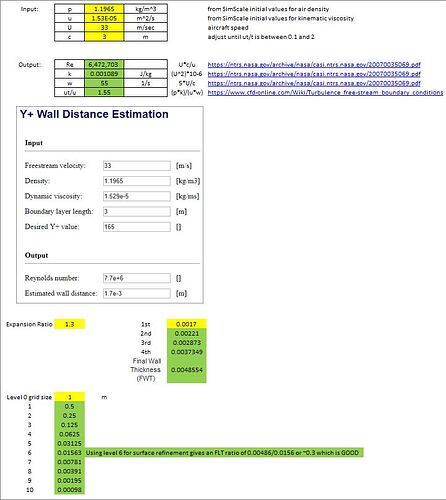
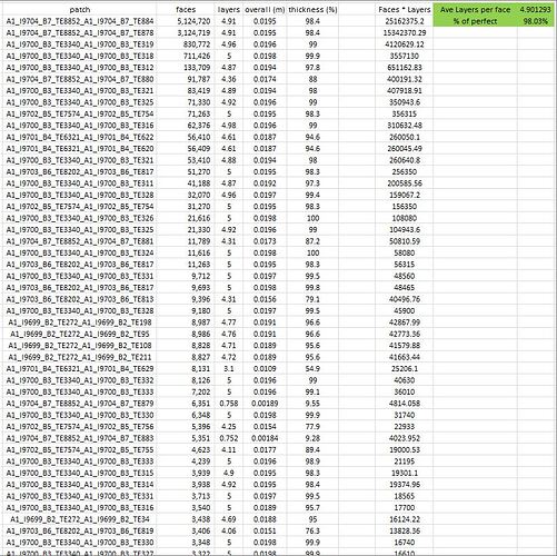
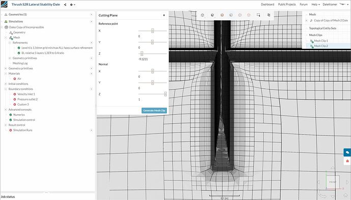
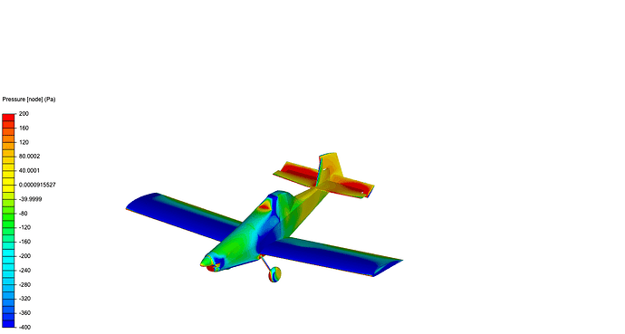
Mesh developed using the Kramer’s Method (oh yeah). Only two refinements: surface and BL inflation. Surface refinement calculated with a target y+ of 165 to be 6 resulted in a nice fine mesh with really good BL coverage (assessing this from the meshing log table). Despite a finer mesh, 4.7MM cells. It’s not how many cells you have, it’s where you put them.
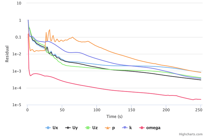
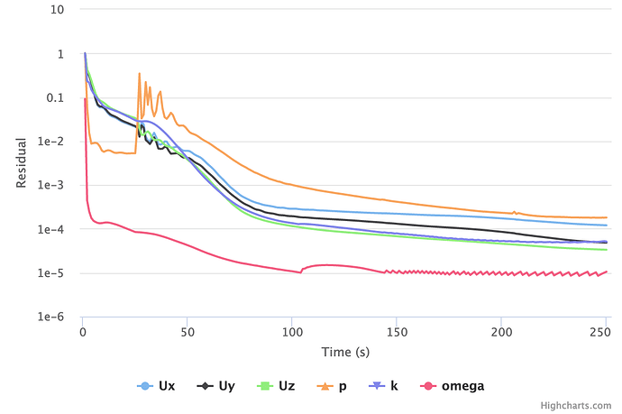
Running identical simulations - velocity ramped over 25s, 1s timestep, the Kramer model converged more quickly. Here is my convergence plot:
And the Kramer plot:
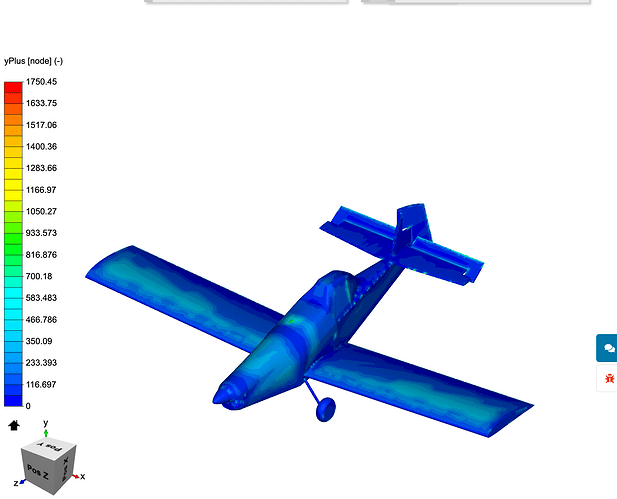
y+ for my model was all over the place, and high:
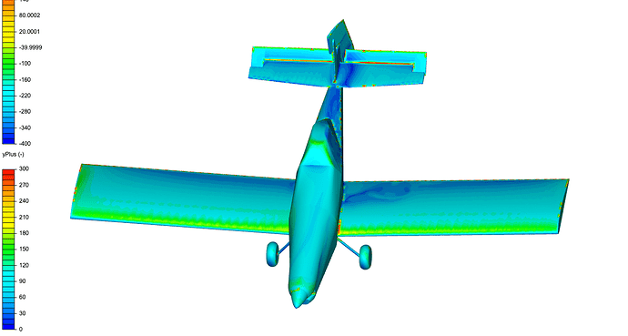
vs Kramer’s (note different scaling):
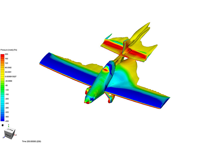
The results speak for themselves. Here’s pressure distribution across the model
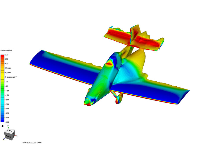
Versus Kramer’s:
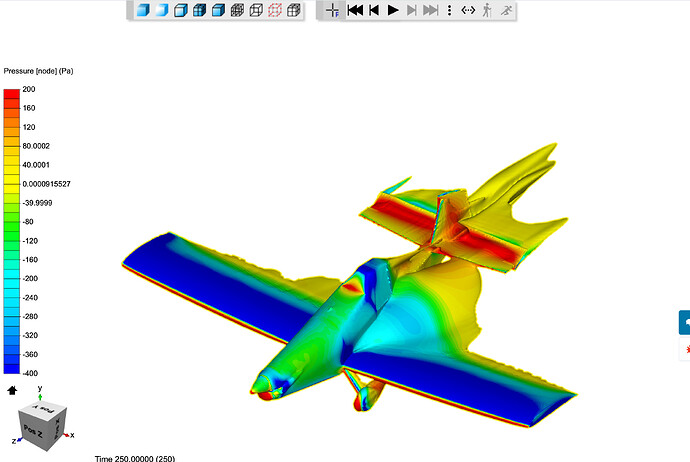
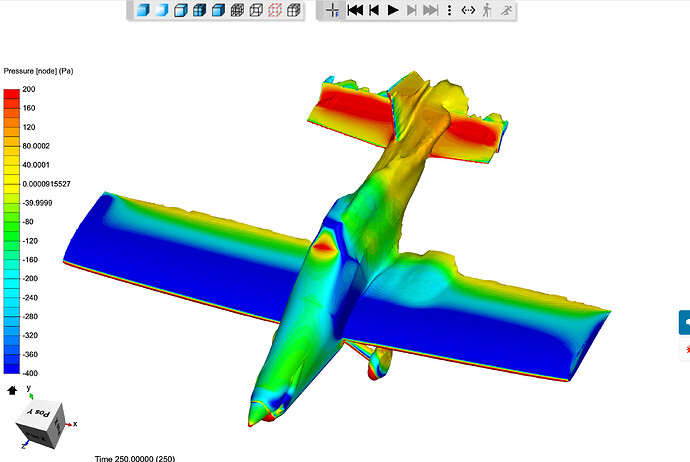
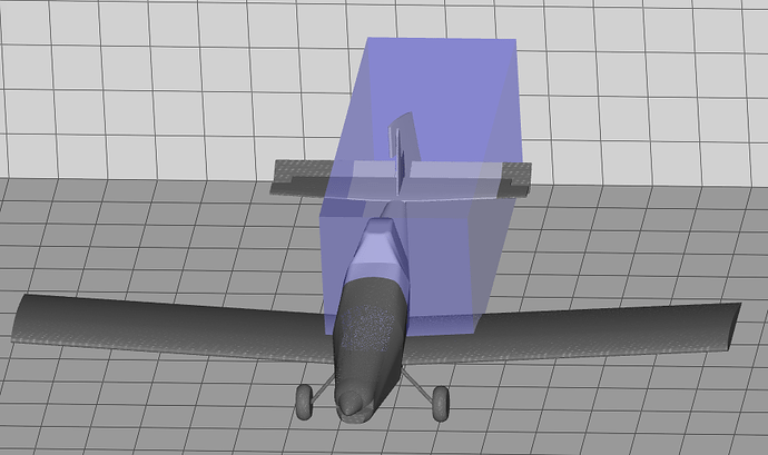
And isovolumes showing ~50% of the freestream velocity and lower. My mesh shows a large recirculation zone beside the fuselage, eventually enveloping the tail midway along the horizontal stabilizer.
In Kramer’s mesh, we see this zone is almost completely absent. The separation caused by the fuselage instead follows the empennage and connects with the tail much further inboard where we can expect it to have much more of an effect on the rudder. This difference was one of the results that had me really puzzled… in my mesh the rudder still appears to be very effective. In Kramer’s it’s much less so:
Okay that’s what I’ve got… now running out of memory trying to bring the surface refinement up so this might be as good as I can do on 16 cores. Next I’ll add some region refinements to Kramer’s mesh to see if I can smooth out the flow field a bit, but until then - HEED MY WARNING 
EDIT
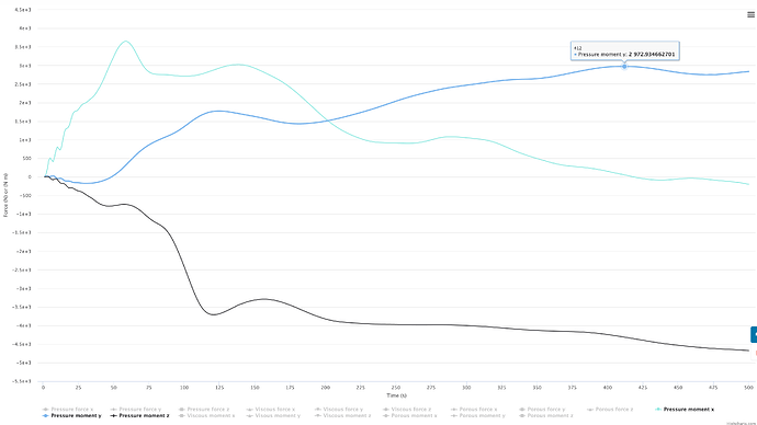
I went ahead and extended the simulation time of the Kramer BL mesh because I had a feeling that it hadn’t achieved steady-state yet. The result is more in-line with what would be expected… similar flows but probably more accurate with a better BL.
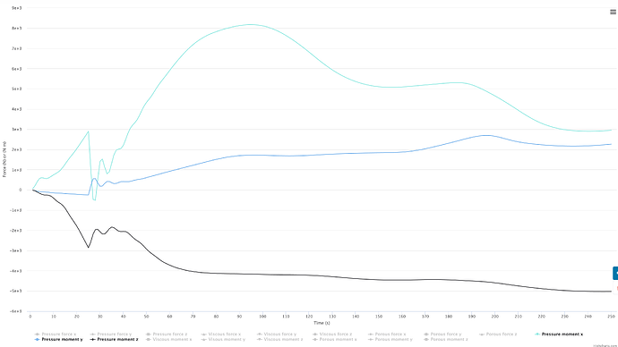
Moments of the poor mesh:
Moments of the Kramer mesh @ 500s:
0-15m/s Z velocity isovolume of the poor mesh:
0-15m/s Z velocity isovolume of the Kramer mesh @ 500s:


