Remotely Operated Vehicle | Drag

[Maciek]

Here we go with a proper software test!

So far I’ve run a series of about 40 simulations for three different vehicle configurations. Some of the runs ended up with a crash obviously, but generally speaking results are… well (at least) very good.

I was a bit hesitant due to all these mesh problems, but ultimately I decided to start this topic and present work I’ve done so far. The reason for this was the fact that despite of imperfect mesh the outcomes have started to be repeatable. While playing with the first vehicle’s configuration and changing both mesh and simulation settings I achieved a state where results matched the experimental data. And when I transferred the mesh and simulations settings to two other configurations simulations delivered very good convergence right away. Below I’d like to present the outcomes together with convergence rate and some short comment.

Also, given my experience in different types of simulations, I know that sometimes you are compromised by geometry or/and conditions and you have no choice but accept the situation. In this particular case I’m aware some regions may be very problematic for mesher and later for solver and obtaining desired mesh there is nearly impossible.

In short: what we have here is an unmanned mine-cleaning underwater vehicle. It is powered in two ways by standard propellers and waterjet drives. Standard propellers are additionally protected by a grill. All the simulations were run for an operational velocity.

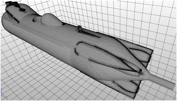
Surface meshes (I left pictures in big format for better view)

ROV Standard Propellers with Grill
aft section

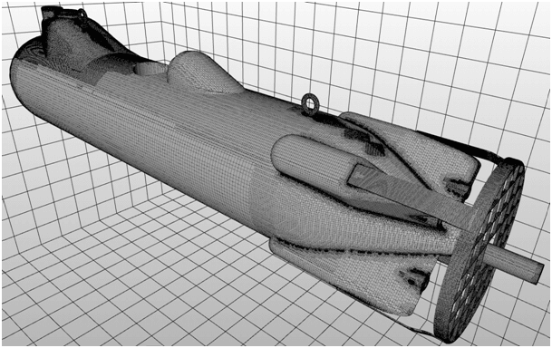
bow section

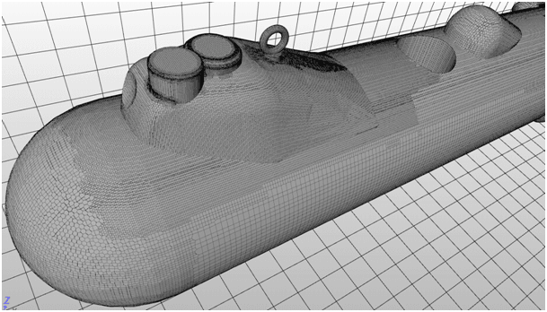
ROV Standard Propellers
aft section

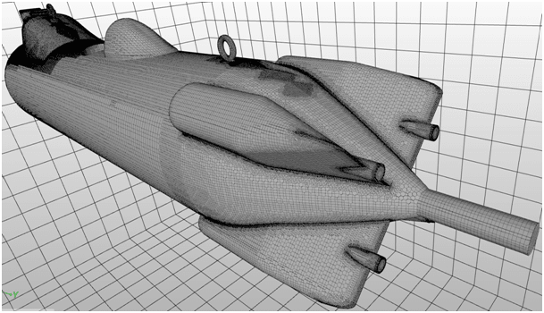
ROV WaterJet Drives 50
aft section

I wasn’t sure how to present outcomes in attractive way. Finally I choose turbulence representation coloured by velocity. I hope it is fine for you.

ROV Standard Propellers with Grill

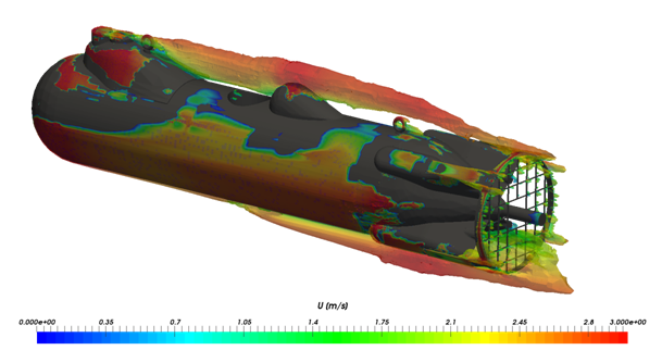
ROV Standard Propellers

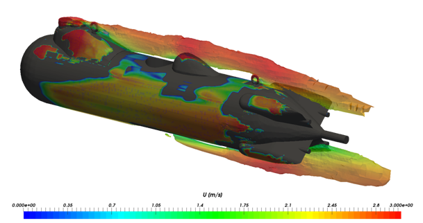
ROV WaterJet Drives 50

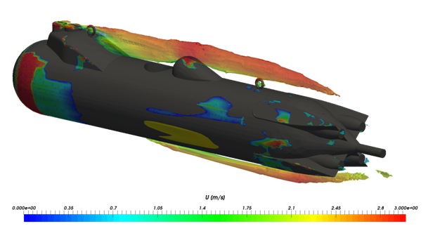
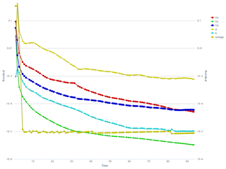
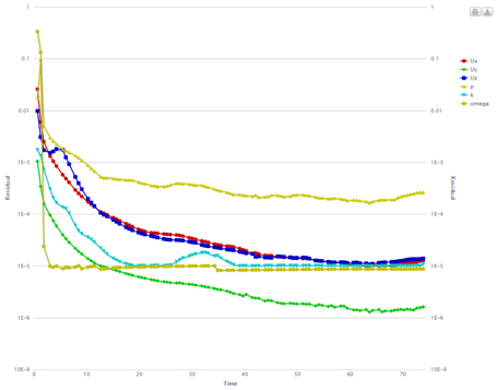
I’d like to add plots too as I have some comments to it:

ROV Standard Propellers with Grill

ROV Standard Propellers

ROV WaterJet Drives 50

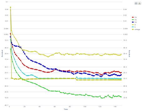
And finally the most important thing – convergence rate:
ROV SP+G -0.2 %
ROV SP -3.8%
ROV WJ50 -%4.7

In conclusion: I’m really happy with the results. Not because the values themselves, but because they proved to be repeatable for different settings. Given the residuals however (which in fact reflect the mesh) I think outcomes for ROV with standard propellers and grill will ultimately be a bit smaller (that is convergence rate will be slightly worse). But generally speaking (writing) overall tendency to gently underestimate vehicle’s drag is proper and should be regarded as positive.

The thing I’d like to work on is better pressure convergence as I found it quite difficult. On some occasions solver suddenly lost stability and case that looked very promising crashed. Of course I know it’s strongly related to the mesh, so I hope improving meshing will automatically improve this.

GENERALLY

1. Progress bar and Runtime counter sometimes freeze showing zero for the duration of the simulation.
2. I don’t know if I wrote it before, but I really like the residuals plots (!). The only thing I’d like to have here is a possibility of saving it as a picture. Best if I could do it with its unusual resolution – compressed plot sometimes blurs the view and tendency.
3. Solver seems to be really solid (!). I would even say that default convergence level set at e-5 is rather strict and e-4 is more than enough. I tested it on simpler cases and I saw no (real) differences.
4. Is there a possibility to set convergence rate as a simulation target instead of time? I mean the only target. I get the idea behind ‘time’, but what if time I’d set was just too short. Is there a possibility to start simulation from the point it ended?
5. What do you think about this strange mesh assignment I described in this topic? Taming relative meshing | snappyHexMesh - #4 by Maciek Should I worry about it? Or it’s just the way that mesher sometimes divides the geometry?
6. Looking at the surface mesh I’m really happy with it. Only this BL…

As you can see the simulations look good at this stage. However if you have any comments or spotted something you think I missed feel free to point it out!

[dheiny]

@Maciek, awesome work! What CAD software did you use? Agreed, the pressure convergence often is challenging. Regarding (2) and (4):

(2) --> Tracked as a feature request and +1 for you
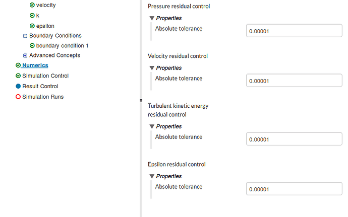
(4) You can find this option under “Numerics” where it says “… residual control” (see image below). Once all residual control values are reached, the solver will end its run and write by default the last time step.

[Maciek]

@dheiny as I’ve written in my report I use academically licensed Solid Edge version 20. It’s the last one without synchronous technology. Program is now nearly a decade old, but it has all basic features I need. What’s more the licence is timeless. Therefore, as long as I don’t make money I can use it however and wherever I want. (For me my PhD project wasn’t commercial one.)

The next project’s geometry however was provided by its designers. (I’m currently working on that electric car. I hope I’ll finish it until the end of this week.)

Residual Control
Yes, I know where to change the residuals’ level and how it works I just thought I could get rid of time factor completely. But I see I should rather set long time for the simulation and control the plots – ok.

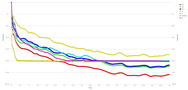
In terms of convergence: I’m a bit confused here. For me velocity and pressure are bonded with each other, so good convergence of velocity should trigger good convergence of pressure automatically. At least that’s how it works in e.g. CFX. The real challenge is to obtain expected convergence for velocity and turbulence at the same time. – Often one of these two goes smoothly and other is more reluctant. Therefore could you explain in few words how it works here?

Also correct me if you think I’m wrong or ask for more if you want me to describe something in more details or in different way.

Simulation Control / Write Control
BTW a silly question about results writing frequency: Runtime is the appropriate option if I need only the first and the last time step?

[Maciek]

Hmm… to be frank I expected some comments, remarks or question so that to start a discussion. Well, if there is nothing like this, than I assume it looks fine to most of you.

However, I felt there is something obvious missing here: accuracy.

The vehicle is set to operate at the open sea, which means unlimited water for it. Obviously there is no possibility to measure anything in such environment, so all drag and propulsion tests were run on the lake – from vehicle’s perspective it is unlimited water. Standard deviation for measurements taken this way was about 8%. But given small values we deal with here I rounded it to full 10% and this is / was my error margin. Of course you have to remember that you add plus-minus sign before this value too! In a result we get 16-20 % error window.

Personally I set myself a goal to get into half of it (10%) and classified it as very good convergence. If simulation outcomes fit in 20% margin I labelled them as acceptable convergence.

Now, I’m aware that for some of you, beloved in motor sport, it sounds ridiculous, but believe me taking measurements of such a small values sitting on a boat is very challenging even if you think the water is calm and the water table flat. Simply, such inaccuracy has to be taken into account.

I hope now you have better view of results presented here and it’s clear for you why I’m satisfied with them despite of a couple of percent of a difference.

[jprobst]

Hi @Maciek,
let me post a quick reply to your questions before we go deeper into the discussion:

@Maciek

Simulation Control / Write ControlBTW a silly question about results writing frequency: Runtime is the appropriate option if I need only the first and the last time step?

Yes, if you set choose Runtime and assign the same values to End time value and write interval, the last time step will be written. The first time step is always written.

@Maciek

In terms of convergence: I’m a bit confused here. For me velocity and pressure are bonded with each other, so good convergence of velocity should trigger good convergence of pressure automatically. At least that’s how it works in e.g. CFX. The real challenge is to obtain expected convergence for velocity and turbulence at the same time. – Often one of these two goes smoothly and other is more reluctant. Therefore could you explain in few words how it works here?

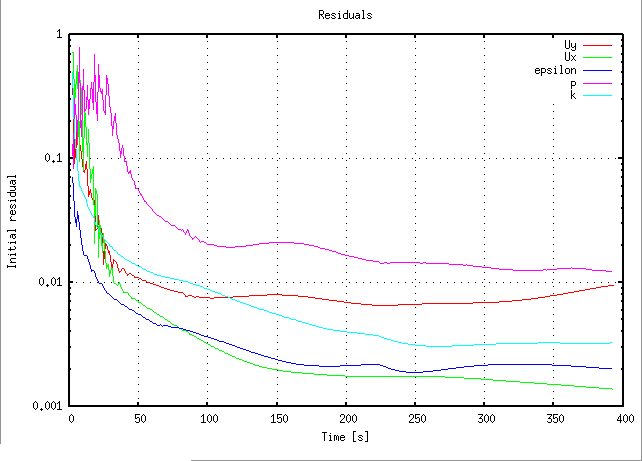
The convergence criteria here mean that we consider the final solution converged if the residuals fall below the threshold for all fields. One thing I saw in your convergence plots is that the omega equation seems to converge extremely fast and its residuals stay at a constant level (10⁻⁵) throughout the simulation. Could you double-check the settings for the linear equation system solver for the omega equation? I believe that its absolute tolerance is set to 10⁻⁵ which will cause it not to perform any iterations at all since this residual is already reached. If so, you could try an even lower tolerance (2-3 orders of magnitude smaller)?

[Maciek]

Hi @jprobst it’s great you’ve joined.

Simulation Control / Write Control / Runtime
I did and… instead of expected 300-400 MB I got nearly 25GB

CONVERGENCE
Yes, you are right I kept convergence criteria (Absolute Tolerance) at level e-5 for all elements.

I also did as you had written, but it changed nothing. Moreover, it sounds a bit strange to me: why is it being solved no longer? I thought the convergence criteria are to trigger solver stop and a case is being solved as long as all the criteria have not been met. Does it work with turbulence only? If we look at the velocity it goes down even if all three reached e-5 threshold.

(These plots come from a compressible case.)

I followed solver’s advice and changed Divergence scheme for U | k | omega from Gauss upwind to bounded Gauss upwind. - I would say it made a difference and improved convergence (mostly stability).

Further I decreased relaxation factors too:
pressure: 0.3
velocity: 0.3
k: 0.5
omega: 0.5

Do you have more questions to me? Something that could help to identify my potential errors? In my opinion the rest depends on mesh – I’m working hard on it.

[jprobst]

Hi @Maciek

@Maciek

I did and… instead of expected 300-400 MB I got nearly 25GB

this is indeed a lot… If you did all the simulations (you wrote 40 different ones) in one project it might have grown up to this size. If not and you don’t mind sharing your project, I can check your setup to see where all that data went. Out of curiousity: how many cells do you have? (you find the info when you click on the Mesh Operation and scroll all the way down in the middle panel to “Mesh Operation Event Log”).

I’d like to join the discussion about the consistent underestimation of drag you’re seeing. First of all: I would also call the accuracy you achieved (-0.2% and -4.7%) “very good”. Some people might think this is a large tolerance (e.g. in aeronautic applications, F1, or regarding the precision needed for a steam turbine in a power plant) but as you descibed, the kind of application and the maximum accuracy in experiments count as well in my opinion. Especially for an ROV, you will probably have changes in water temperature, mud, algae, currents and so forth, which have big impact on its operation, too.

You’re mentioning 2 potential sources:

1. solver tolerances and convergence criteria
2. mesh

Let’s start with 1, solver tolerances and convergence criteria.

@Maciek

Moreover, it sounds a bit strange to me: why is it being solved no longer? I thought the convergence criteria are to trigger solver stop and a case is being solved as long as all the criteria have not been met. Does it work with turbulence only? If we look at the velocity it goes down even if all three reached e-5 threshold.

Convergence criteria (called “residual control” on SimScale), depicted by @dheiny in his post Remotely Operated Vehicle | Drag - #2 by dheiny tell the solver when to stop completely. They are normally used with steady-state solvers and terminate the entire computation if all residuals have fallen below the threshold and the solution is assumed converged.

There is another criterion, applied at each time step (or pseudo time step in steady-state simulations). These are the equation system solver tolerances which apply to each equation. If the initial residual for an equation (e.g. omega) is already below the threshold (in this case 1e-5) then this solver will not do any iterations. The other solvers (e.g. p) will still iterate until the final residual reaches the absolute tolerance or if the quotient between final and initial residual has reached the relative tolerance.

@gholami what do you think?

Earlier, you stated:

@Maciek

3. Solver seems to be really solid (!). I would even say that default convergence level set at e-5 is rather strict and e-4 is more than enough. I tested it on simpler cases and I saw no (real) differences.

This indicates that the levels of residuals are fine…

This brings us to point 2, the mesh. Since you say that the drag is consistently predicted too low, I think that the problem could come from the boundary layers. If the boundary layers are meshed too coarse, the velocity shear gradient (and hence the wall shear stress) cannot be predicted correctly. You can use the y+ result control item to check if the mesh is adequately resolved near the wall. Y+ on the ROV’s outer surface should be between 30 and 100 if wall functions are used. If no wall functions are used, you should have a y+ < 1.

But your results are impressive anyways so I think we shouldn’t really speak of an “error” in this case. It looks like you’re not doing anything wrong.

[gholami]

Hi guys,

this is a very interesting topic. Firstly, @Maciek you’ve created quite a case. Your mesh and results look good. I even think the accuracy you get is absolutely OK considering the complexity of the geometry. Well done!

Regarding the discussion on convergence plots, @jprobst already mentioned the two key elements:

Residual control:

@jprobst

tell the solver when to stop completely. They are normally used with steady-state solvers and terminate the entire computation if all residuals have fallen below the threshold and the solution is assumed converged.

Absolute tolerance:

@jprobst

applied at each time step (or pseudo time step in steady-state simulations). These are the equation system solver tolerances which apply to each equation. If the initial residual for an equation (e.g. omega) is already below the threshold (in this case 1e-5) then this solver will not do any iterations.

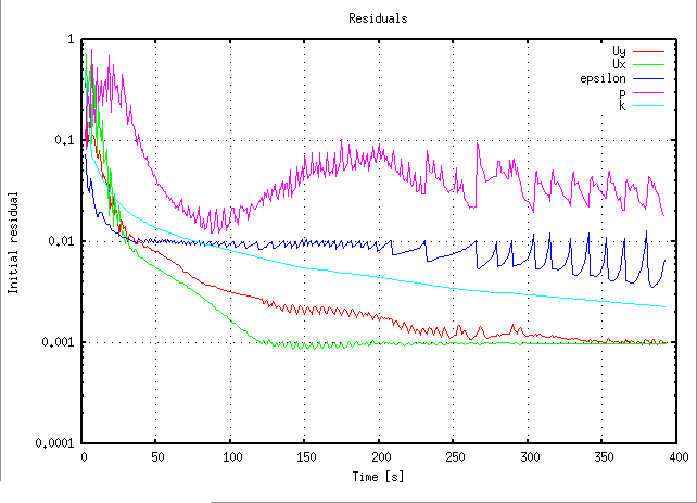
In other words, absolute tolerance only belongs to the solver’s inner loop where each variable is being solved. When residual is below the absolute tolerance, no inner loops will be performed. To show how this could be relevant to your case, I’ve created two simulations:

The only difference between these two simulations is the absolute tolerance for epsilon; 0.01 for the top case, and 0.001 for the bottom. As you see, the convergence behavior differs substantially between the two cases. In the top case, epsilon equation reaches “convergence” way too early in the simulation for other variables to adapt. So, the tolerance must be chosen carefully.

My take on this is that you could try to decrease the absolute tolerance of omega, to e.g. 10⁻⁶, to see how the convergence behavior and the final result change. Apart from that, it is not unusual for a variable’s residual to decrease below the threshold while the rest of the variables are still being solved.

In the end, it would be useful to know more about the simulation. We might be able to dig more into it. Let us know if you worked on your simulation further. I’m interested to see if results improve even more.

[Maciek]

@jprobst @gholami

Hi Babak and Johannes and thanks for your posts. Also sorry for my late response, but here we go:

RESULTS’ FILE SIZE
As it’s easy to guess I already deleted it I don’t know what went wrong, but ultimately decided to stick with manual determination each time (total run time divided by time step).

You may be right and all meshes, pre-processor definition files and results files could just pile up together as I keep it all in one project directory. On the other hand, using manual approach I’ve never encountered such situation. I’ll let you know if I hit it one more time.

ACCURACY
I’m happy with regular underestimation. As you mentioned simulation doesn’t include elements such mud, underwater current, random dirt and scratches on hull surfaces etc. - hence the scatter in experimental outcomes and nearly 10% measurement accuracy.

Two curious details:

1. vehicle’s handlings alone (the two rings at the top of the ROV) increase the total drag by about 10% in comparison to the vehicle without them
2. the grill increases the total drag by 45-50 %.

BOUNDARY LAYER and Y+
Yet again I see we understand each other very well. I also think mesh and Boundary Layer in particular is the region where I should look for any gains. I know the mesh is imperfect (I run separate topic with it here Taming relative meshing | snappyHexMesh ), but I encountered similar problems in other software too. – BTW I think it’s a very good example of difference between solving theoretical and real problems. In real problems often something unexpected causes big troubles and compromises final solution.

Generally speaking it’s very difficult to meet Y+ requirements in some regions - for instance the handlings. These two rings need really dense mesh to map the surfaces properly and at the same time are so small that, inside their geometry, they can hardly contain required BL.

This is the reason why I had to turn the blind eye at some regions and why I decided to publish the outcomes despite all this imperfections. My judgement was based on results repeatability for different mesh settings.

Of course I still believe we’ll find some solution and / or explanation for mesher behaviour.

In terms of Y+ values for particular cases they are up to:
ROV SP+G: 210
ROV SP: 180
ROV WJ50: 250

I’ve run the simulations with a use of SST model, so reference range is 20-200 (or 30-300 as some may say). If we look at the theory the transition point for wall function in this model is at value 11.28 (or 11.68 I can’t remember this precisely). Anyway it’s easy to remember the number is flat 12. For safety reasons we move it up to at least 20.

The upper limit, theoretically, doesn’t exist, but operating with thousands or more – from my experience – can be deceptive and it’s better to keep values at hundreds range.

In my cases the overall layouts are not perfect (due to reasons mentioned in separate topic), but they still look ok(ish). Of course the regions with very high refinement (e.g. bended corners) go below 12, but I’m afraid I have no choice but accept it.

MESH COUNT
Mesh count here is much higher than I expected. But I think it’s all due to cut-cell mesh. A kind of price you have to pay for its regularity. The reference count for mesh elements was about 2.5 million and for nodes up to 1 million. What we have above is:
ROV SP+G: ~13.9 mln elements and ~5.17 mln nodes
ROV SP: ~7.75 mln elements and ~2.9 mln nodes
ROV WJ50: ~9.15 mln elements and ~3.5 mln nodes

Personally I wouldn’t complaint about it. At some areas the mesh may look a bit too dense, but on the other hand it’s nice and regular. I see it this way: in 2D tetramesh when you want to coarsen or refine your mesh you just add an element a bit deformed in comparison to the previous one (slightly bigger or smaller). And you can control step size too. In cut-cell however the step is always ‘2’ (or 100% if you prefer this labelling). Anyway I prefer this approach even if simulation lasts longer.

ABSOLUTE TOLERANCE
(My account yet again switched to free mode and at the moment I can’t do anything, but as soon as Agatha fix it ) I’ll experiment with the settings more and let you know if and what influence on residuals it has.