Tutorial Updated 2018-01
Recording
Introduction
The FEA Master Class: Session 2 underscores the significant impact that the material has on the outcome of the simulation. In this exercise, you will be enabled to utilize the SimScale Platform to setup a Finite Element Analysis (FEA) study to simulate the forces on a child’s bicycle wheel, if a sumo wrestler sits on it.
The stress-strain curve describes the behavior of a material under loading. The primary aim of this analysis is to study the non-linear plasticity effects on a wheel rim and determine the role played by the material type on the physical significance of the result.
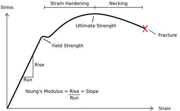
Hence, our analysis is to be done post the yield strength point (non-linear region) of the wheel rim material, i.e., Polypropylene.
Import Project
Given below is the link to the initial point of the project:
Handout Project: Project Link
Now that you have been provided with the Bike Wheel Geometry (wheelFEA), you can use it to set up a simulation that analyzes the effect of the material type on the results.
Mesh Generation
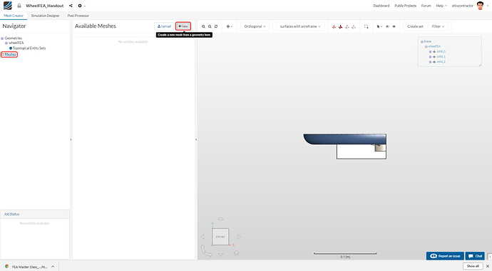
Start up the Mesh Creator mode in the workflow. Select the Meshes in the Navigator and click on New to begin with the meshing procedure.
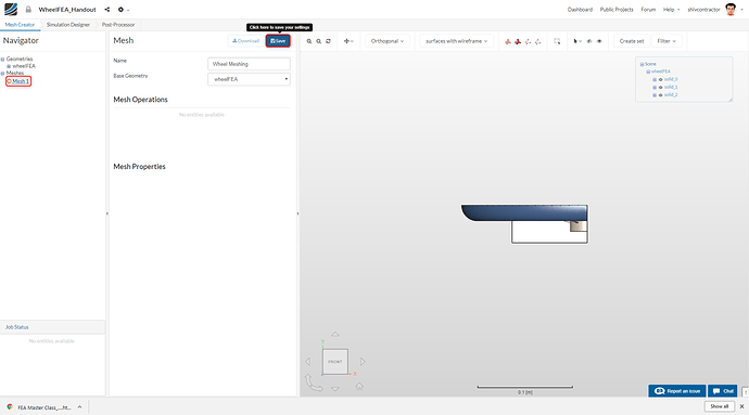
After assigning an appropriate Name to your mesh, select the Base Geometry as wheelFEA.
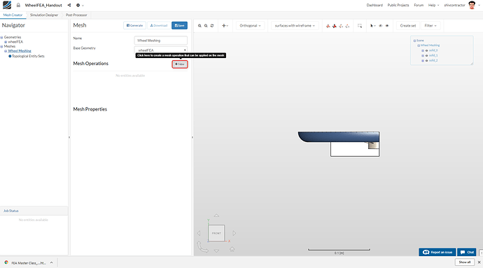
Please a new Operation by clicking on New.
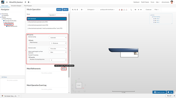
A Tet-dominant mesh operation is used for this FEA study. The global mesh sizing may now be set as follows:
You may now proceed to make a mesh refinement by clicking on New in the Mesh Refinements tab below.
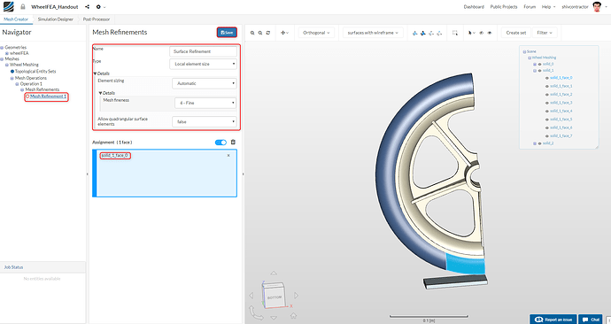
With the intention of refining the surface, which is in contact with the ground, you can follow these steps:
Set the Type as Local element size and the** Element sizing** as Automatic. The Mesh fineness should be 4-Fine. To select the desired face, first, click on the Pick Faces tool displayed on the top of the viewer and then click on the face as shown below. Proceed by clicking Save.
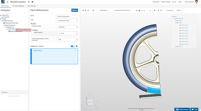
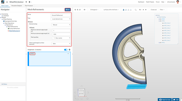
Essentially, the ground is an immovable rigid support on which we do not want to perform any calculations. Thus, we assign it the coarsest mesh possible. To make a new mesh refinement, right click on Mesh Refinements and select Add mesh refinement.
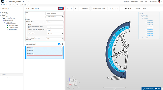
To avoid numerical divergence in the solver, it is imperative that the contact between the rim and the tyre has an identical mesh refinement. This is the intent of our Contact Refinement.
Add new mesh refinement following the procedure described previously.
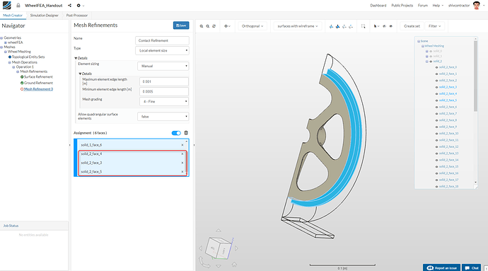
Set the values as shown in the column (Figure 11). On the top right of the viewer, you will be able to see a Show/Hide box. Hide solid_0 and solid_2 by clicking on the Eye Icon next to them. The hidden items will be rendered transparent and the shown ones will still be colored. Now, you can easily select the three faces of the tyre as shown in the image below.
Subsequently, hide** solid_0** and solid_1 and show solid_2. The three faces of the rim which are in contact with the tyre should be selected. Use the same mesh refinement specifications as earlier.
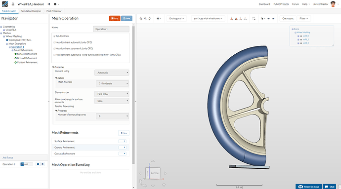
Click Save after the global meshing and 3 local refinements have been setup. Open the Operation 1 tab and Start the mesh operation.
The meshing can be tracked from the progress bar shown below.
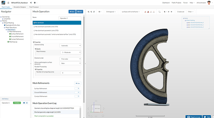
The mesh may now be visualized in the viewer.
Kindly note: Confirm your mesh specifications with the ones shown in the image below before starting the Mesh Operation
Simulation Setup
Select the Simulation Designer tab in the workflow and click on New to create a new simulation setup.
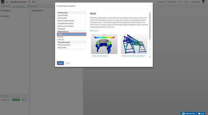
You will see an array of simulation types you can choose from. In our case, we choose the Static simulation under the category- Solid Mechanics
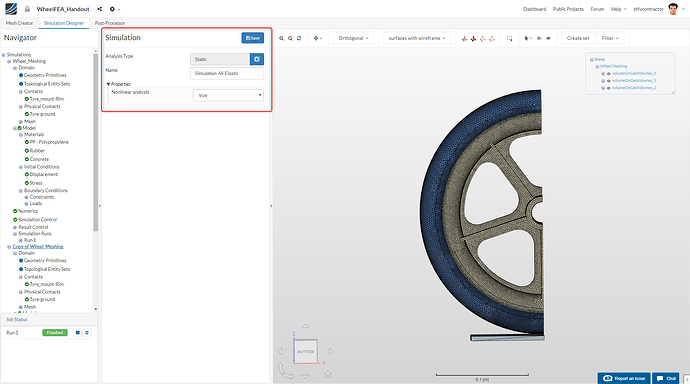
Please assign an appropriate name to your simulation and set the Nonlinear analysis to** true**. This is because we want to study the non-linear plasticity effects on the wheel.
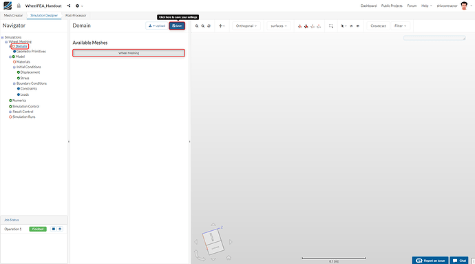
Select Domain from the Navigator. You will be able to see the mesh that you have created. Select the desired mesh on which the simulation is to be performed.
The mesh will be displayed on the viewer as shown in the figure below. Click Save to continue to the simulation set up.
Contact Defnition
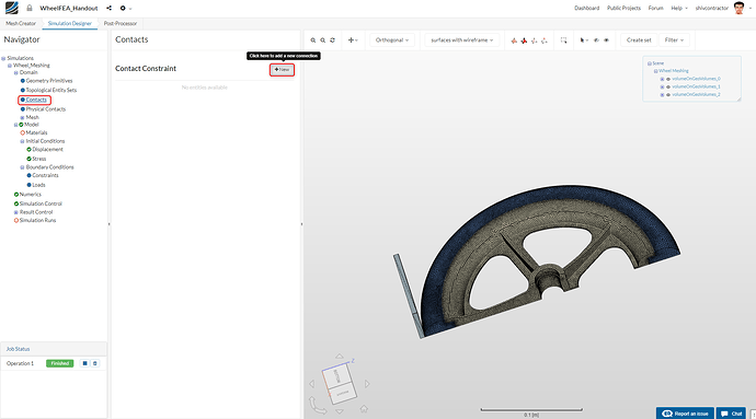
Let us move on to assigning the contacts. Select Contacts in the Navigator and create a New contact
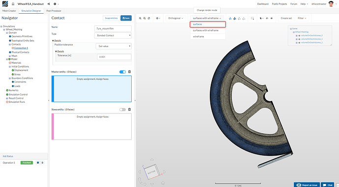
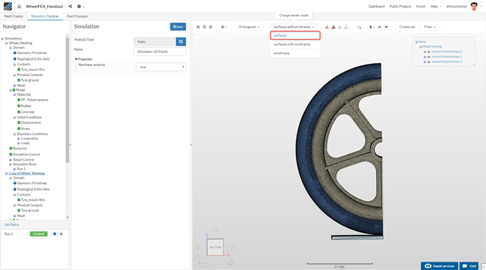
Change the render mode to surfaces to proceed with the simulation setup.
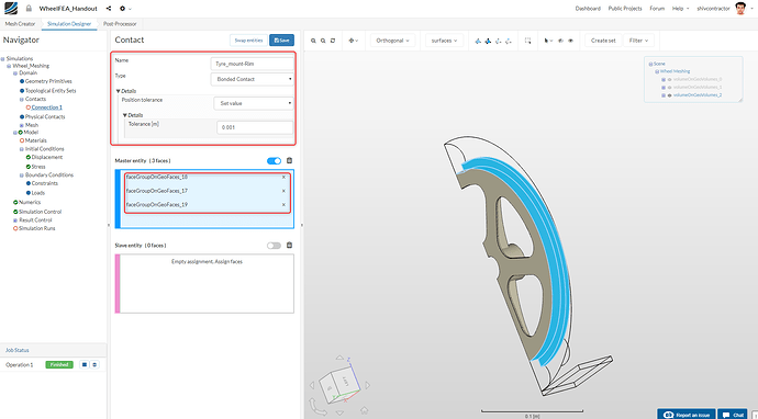
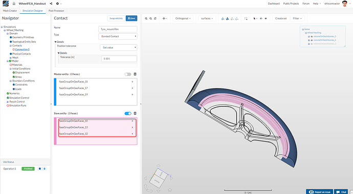
Generally, it is considered to be a best practice to select the more rigid material as the Master Entity. In our case, that would be the rim. Select the faces of the rim that are in contact with the tyre. Moreover, change the Type of Contact to Bonded Contact and the Tolerance to ** 0.001**.
Similarly, assign the surfaces on the tyre that are in contact with the rim as ** Slave Entity**.
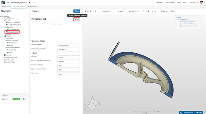
Since we intend to perform a static analysis, we assume that the contact between the tyre and the ground is set as a frictionless physical contact. Select the Physical Contacts option in the Navigator and create a New physical contact.
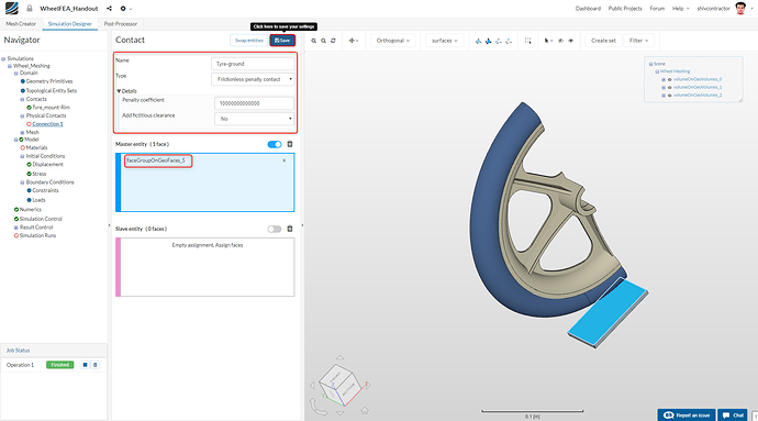
Select the Type as Frictionless Penalty Contact and increase the Penalty coefficient to 10000000000000 (10e+13). As you already know, the more rigid body should be assigned as the master entity. As we’re dealing with the contact between the tyre and the ground, the ground would be the Master Entity.
Kindly Note: Make sure that you use to the face selection tool to select only the surface of the ground which is in contact with the tyre and not the entire volume.
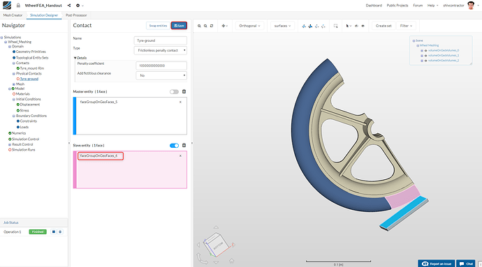
Likewise, assign the surface of the tyre that is in contact with the ground as the Slave Entity.
Material Selection
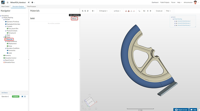
Choose the Materials option in the Navigator and click on New
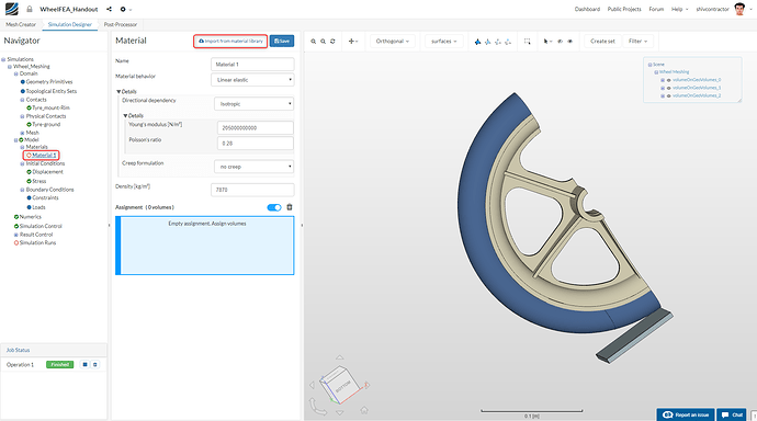
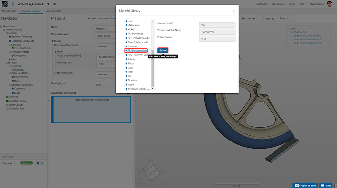
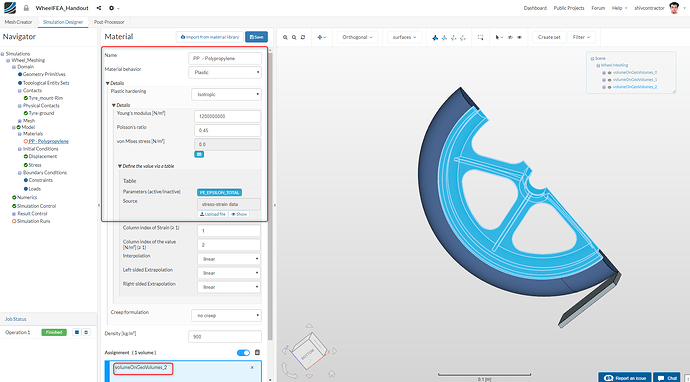
We need to assign the material Polypropylene to the wheel rim. To do this, click** Import from material library** select PP-Polypropylene from the list of Materials displayed in the library.
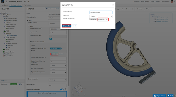
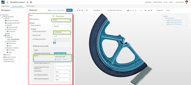
Since we intend to study the plasticity effects in the rim, the Material behavior should be set to Plastic. Please note that this would be our first varying parameter for the next simulation. Set the Young’s modulus to 1200000000 (1.2 GPa).
Next, upload the required .csv file to the platform. This file contains the stress and strain data which defines the plastic behavior of the material. The prepared .csv file can be obtained from here.
The steps are illustrated in the images shown below:
This material is now mapped to the rim by selecting it in the viewer using Pick Volumes.
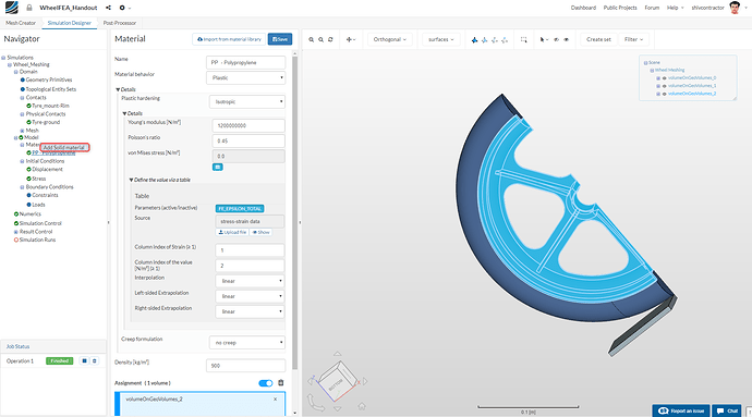
To add a new material, right click on** Materials** in the Navigator and click on Add Solid material.
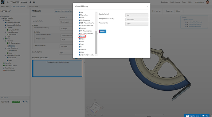
You may now import the material Rubber from the Material Library by clicking on Import from material library and selecting Rubber.
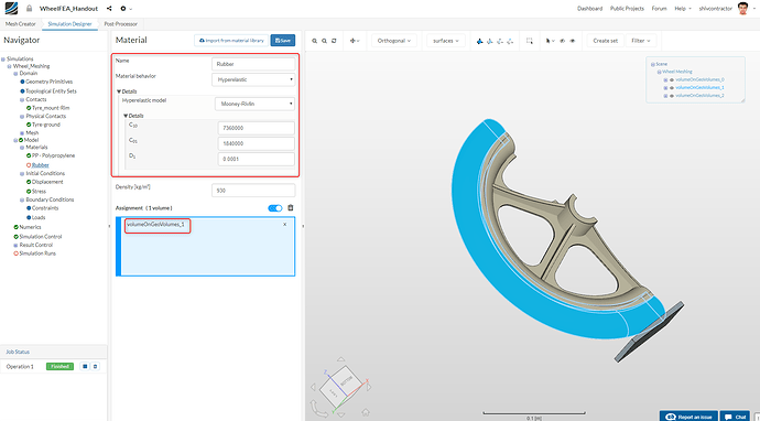
Set the material behavior to Hyperelastic, which is a more accurate representation of the physical behavior of rubber under loading. The Hyper-elastic model is set to Mooney-Rivlin. Please note that this would be our second varying parameter for the next simulation. This material is assigned to the tyre by selecting it from the viewer using Pick Volumes.
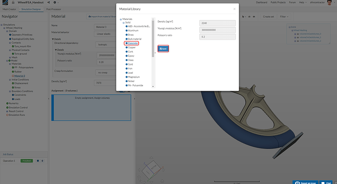
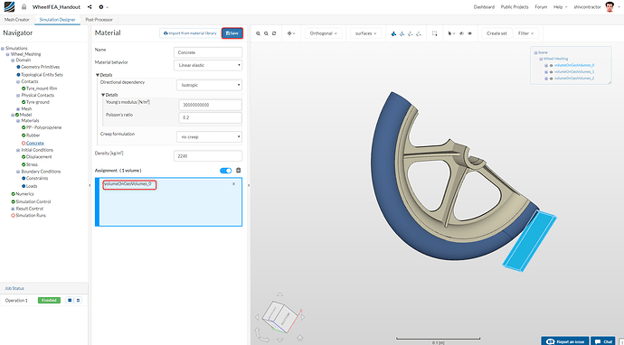
Now, we move on to assigning a material to the ground. As shown earlier, import new material from the library and choose Concrete.
Assign the material to the ground by selecting it from the viewer and using ** Pick Volumes**.
Assigning Constraints and Loads
Here is an overview of the constraints and loads on the Wheel:
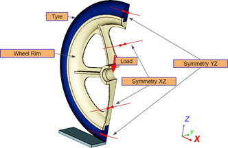
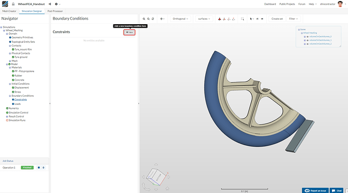
Let us proceed to add constraint boundary conditions. Select Constraints in the Navigator and click on New.
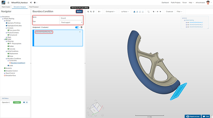
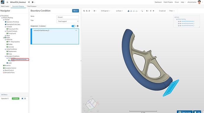
Now, we model the ground as per requirement. Set the type to** Fixed Support**, pick the Ground volume and click Save.
To add a new constraint, right click on Constraints in the Navigator and select Add Constraints bound. You could also click on Constraints and then New to add another constraint.
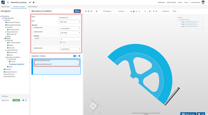
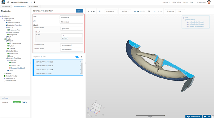
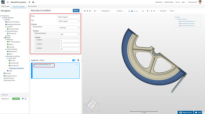
Please follow the settings shown in the screenshots below to model the required boundary conditions.
- The Symmetry in the XZ Plane:
- The Symmetry in the YZ Plane:
- The orthotropic Elastic support:
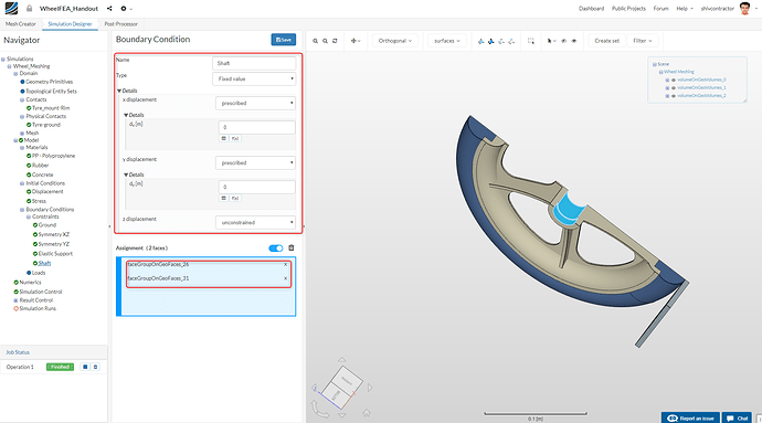
- Shaft Constraint: The influence of the shaft and bearing on the wheel are modeled with the Shaft constraint
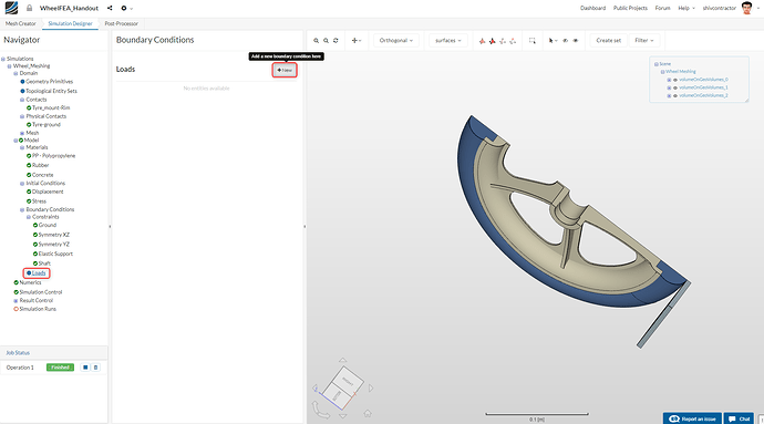
To create a new load, select Loads in Navigator and click on New.
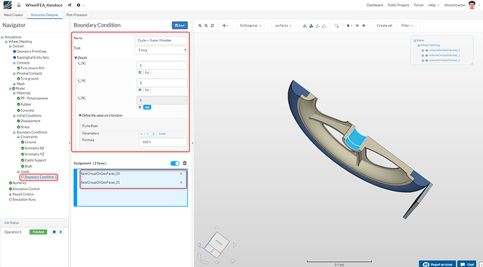
The load on the wheel is modeled with the Cycle + Sumo Wrestler constraint
Click on f(x) in the fz [N] option to select a time-variant force. Add the formula, -505*t, which governs the magnitude and direction of the force. Select the two internal faces which are in contact with the shaft.
Numerics
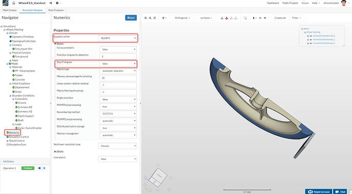
Subsequently, navigate to Numerics and select the solver MUMPS. Set the parameter Stop if singular to false. This is done for the solver to prevent divergence in the initial iterations.
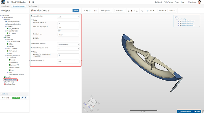
Simulation Control
Select Simulation Control in the Navigator and change the settings to those shown in the image below:
Result Control
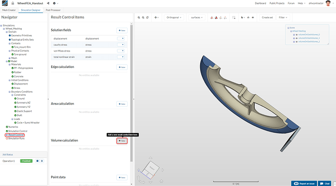
For an effective analysis of the results, it is imperative to monitor the solution fields with Result Control Items. This can be done as follows:
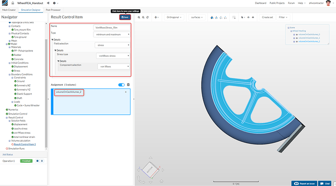
After assigning an appropriate name, set the Type to minimum and maximum. Select Stress, von Mises Stress and von Mises as the subsequent settings. Pick the wheel rim volume to assign it this Result Control Item.
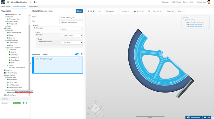
To add a new Result Control Item, right click on Volume Calculation in the Navigator and select Add Volume Calculation.
As done earlier, assign an appropriate name and follow the settings as shown in the figure below.
Initiating the Simulation
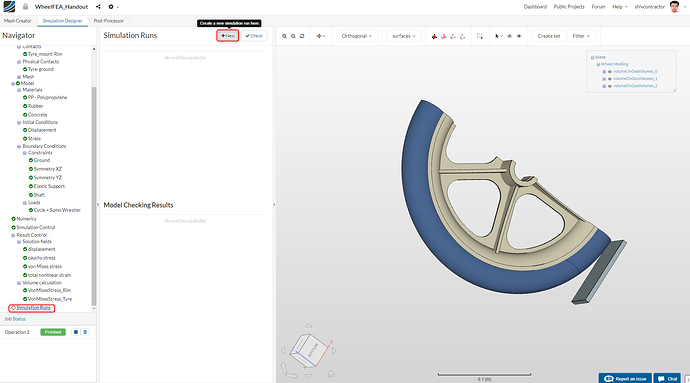
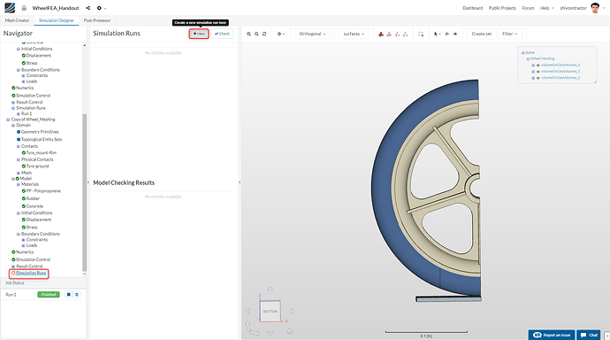
You’re all set to start the simulation. Create a new run by selecting Simulation Runs in the Navigator and clicking on New. Now, you may Start the run.
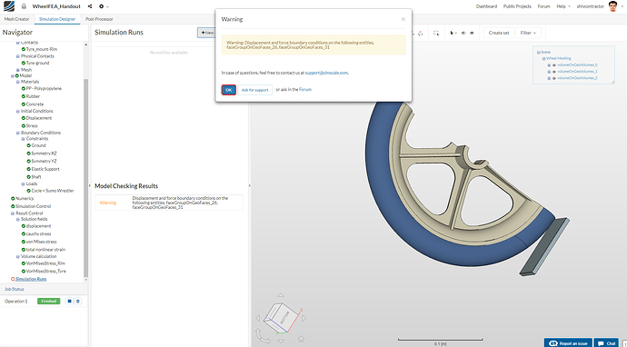
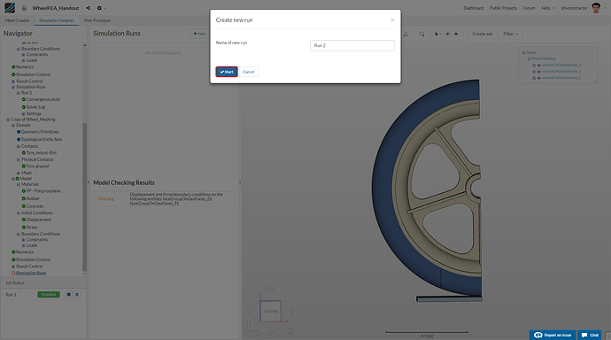
Kindly note: You may receive the following warning when creating a simulation run:
“Warning: Displacement and force boundary conditions on the following entities. faceGroupOnGeoFaces_31, faceGroupOnGeoFaces_26”
You may ignore this warning and proceed to the simulation by clicking OK.
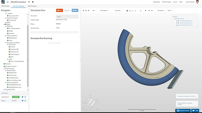
You may Name the run as you like and Start the simulation.
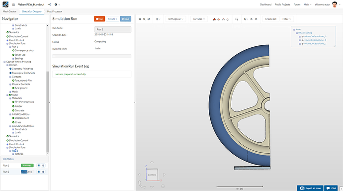
The simulation progress can be tracked in the bottom left of the viewer.
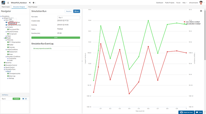
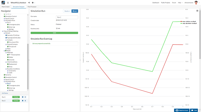
Post the simulation run, you will be able to see this plot and the total time taken for convergence. In case you wonder why it is taking so long, you may note that the simulation takes approximately an hour to converge.
This is due to the mesh refinement.
2nd Simulation set up
To duplicate your simulation setup, go to your first simulation in the Navigator, right click on it, and select Duplicate.
After assigning an appropriate name to your simulation, click Save.
Again, change the rendering mode to surfaces for better visualization.
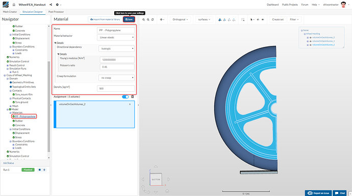
The 2nd simulation is similar to the 1st simulation except in a few regards. In this simulation, all the materials are treated as Linear elastic. You can follow the changes shown in the image shown below to set up your second simulation. Under Materials, change the Material behavior of PP-Polypropylene to Linear elastic. Also, make sure the Young’s modulus is set correctly.
Next, change the Material behavior of Rubber to linear elastic.
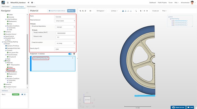
Maintain the behavior of Concrete as set in the previous simulation (linear elastic).
Create New Simulation, name it, and Start.
The simulation progress can be tracked as shown in the figure below.
After completion of the simulation, the following plot will be displayed onto your screen:
Post-Processing
To begin with, open the Post-Processor in the workflow.
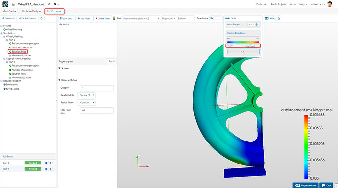
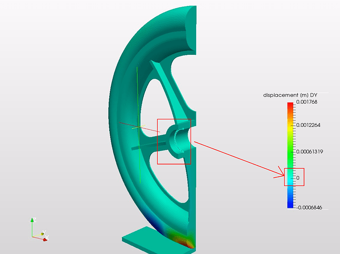
You may now see the result in the viewer, by clicking on Run 1 (or whatever name you had assigned to it) and the selecting Solution Fields. In order to identify the regions undergoing high strain, the displacement may be visualized. Also, it would be a good idea to rescale the custom data range to the values shown in the image below.
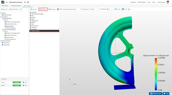
Now, add a filter (Warp by Vector). This will enable you to better visualize the displacement of the wheel under loading. It may be added as follows:
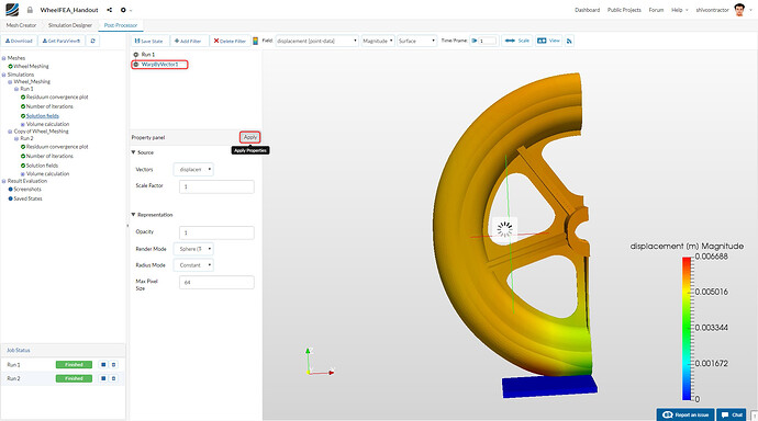
Click Apply to activate the filter. The image below shows the rendered image after the filter is applied.
Once the filter has been applied, you may reduce the Opacity of Run from 1 to 0.5. This will give a clearer representation of the displacement occurring. Change the Field to Solid color and click Apply.
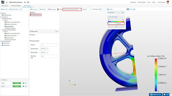
Next, we can obtain the stress contours by switching back to WarpByVector1 and the field to von Mises stress [point-data]. Moreover, adjust the scale to the one shown in the image below.
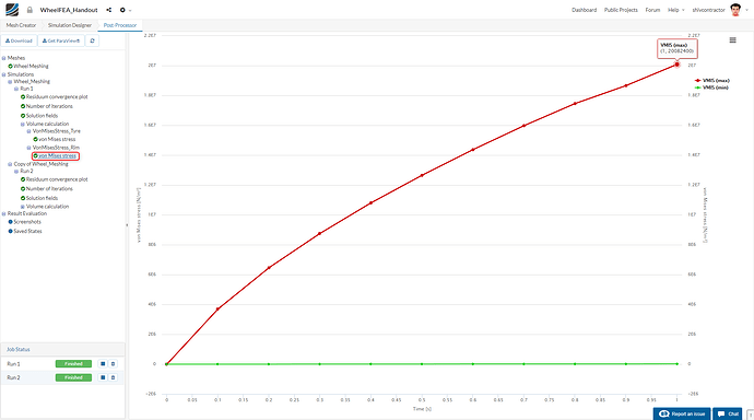
To graphically represent the variation of von Mises Stress with time, click on Volume calculation and then vonMises stress under VonMisesStress_Rim. The maximum Von Mises Stress can be seen by hovering over the topmost point of the plot.
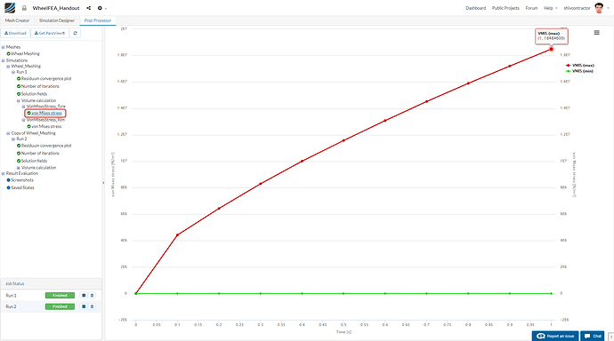
Similarly, the von Mises Stress for the tyre can be plotted by clicking on vonMises stress under the VonMisesStress_Tyre option.
The maximum loads acting on the tyre and the rim can be analyzed with the help of respective von Mises Stress Plots.
Kindly Note: The maximum range is scaled down to 18 MPa, which is the yield strength of Polypropylene. This enables us to accurately visualize the regions undergoing plastic deformation.


