Linear Elastic Materials

A linear elastic material is a mathematical model used to analyze the deformation of solid bodies. It is useful to compute the relation between the forces applied on the object and the corresponding change in shape. In other terms, it relates the stresses and the strains in the material.

For a deformation process to be considered linear and elastic, the following conditions must be met:

• The deformations, in terms of the material strains, are small.
• When the loads are removed, the material naturally returns to its original, undeformed shape. In other words, the material stress level doesn’t reach the yield strength limit.
• The magnitude of the deformations are proportional to the applied loads.

A linear elastic material can be seen as the generalization of Hooke’s law for a spring:

$$ F = Ku \tag{1}$$

where:

• \(F\) is the tensile force applied to the spring,
• \(u\) is the resulting elongation of the spring, and
• \(K\) is the stiffness constant, a property of the spring dictated by the material and geometry.

In order to get rid of the geometry dependency of the stiffness, for the sake of generalization, the relation between force and deformation is expressed in terms of stress and strain:

$$ \sigma = \frac{F}{A} \tag{2}$$

$$ \varepsilon = \frac{u}{L} \tag{3}$$

where:

• \(\sigma\) is the normal stress on the prismatic object under tensile load: force per unit area,
• \(\varepsilon\) is the strain in the material: deformation per unit length,
• \(A\) is the constant cross-section area of the object, perpendicular to the load, and
• \(L\) is the length of the object in the direction of the load and deformation.

By using these terms, the one-dimensional linear elastic relation can be expressed as:

$$ \sigma = E \varepsilon \tag{4}$$

where \(E\) is the Young’s modulus of the material, the proportional relation between stress and strain:

Linear Elastic Materials in Three Dimensions

In the general case of a solid object subject to loads in multiple directions in space, the one-dimensional relation presented above is no longer sufficient to describe the deformations. In three dimensions, stress and strain are expressed as tensor quantities:

$$ \sigma = \begin{bmatrix} \sigma_{xx} & \tau_{xy} & \tau_{xz} \\ \tau_{yx} & \sigma_{yy} & \tau_{yz} \\ \tau_{zx}& \tau_{zy} & \sigma_{zz} \end{bmatrix} \tag{5} $$

$$ \varepsilon = \begin{bmatrix} \varepsilon_{xx} & \frac{1}{2}\gamma_{xy} & \frac{1}{2}\gamma_{xy} \\ \frac{1}{2}\gamma_{yx} & \varepsilon_{yy} & \frac{1}{2}\gamma_{yz} \\ \frac{1}{2}\gamma_{zx} & \frac{1}{2}\gamma_{zy} & \varepsilon_{yy} \end{bmatrix} = \frac{1}{2}(\nabla_X u + \nabla_X u^T) \tag{6} $$

Where \(\nabla_X\) is the gradient operator computed in the undeformed configuration and \(u\) is the vector of deformations in the material:

$$ u = \begin{bmatrix} u_x \\ u_y \\ u_z \end{bmatrix} \tag{7} $$

The general form of the stress-strain relation can be written as:

$$ \sigma = \frac{E}{1+\nu} \Big( \varepsilon + \frac{\nu}{1 – 2\nu} Tr(\varepsilon) I \Big) \tag{8}$$

Or solved for the strain:

$$ \varepsilon = \frac{1 + \nu}{E} \Big( \sigma – \frac{\nu}{1 + \nu} Tr(\sigma) I \Big) \tag{9}$$

where \(\nu\) is the Poisson’s ratio, which relates normal stresses with deformations in the perpendicular directions. Here, it is assumed that the material is isotropic and homogeneous, which means that the material properties such as \(E\) and \(\nu\) are constants with respect to position and orientation.

Workbench Setup

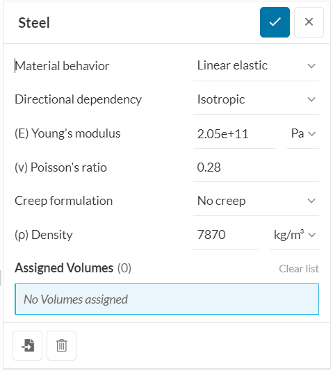
For the application of a linear elastic material in a structural simulation, the following set of parameters must be specified:

• Young’s modulus \((E)\)
• Poisson’s ratio \((\nu)\)
• Density \((\rho)\)

In the Workbench, go to Materials, confirm the Material behavior to Linear Elastic, set the successive parameters and assign them to a volume:

Related Projects

Tutorial: Stress Analysis of a Crane

Validation Case: Design Analysis of a Spherical Pressure Vessel

Last updated: May 26th, 2021