websights

Fill out the form to download

Required field
Required field
Not a valid email address
Required field
Required field
  • Set up your own cloud-native simulation in minutes.

  • Documentation

    Temperature Fixed Value

    With the fixed temperature value boundary condition, a prescribed constant or variable temperature value can be applied to the assigned entities (faces or volumes). This is useful to model constant temperature heat sources or sinks, or to apply a known spatial distribution of the temperature field.
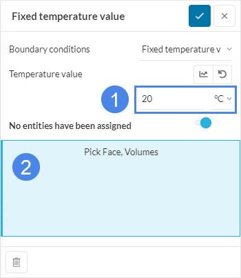
    fixed temperature boundary condition panel
    Figure 1: Fixed temperature value boundary condition panel. Enter the desired temperature and units, or select the variable button to input a formula or table.

    The parameters of the boundary condition are:

    1. Temperature value: The value of the temperature variable to be applied.
    2. Assignment: Set of volumes or faces where the fixed value will be applied.

    Application Hints

    • Do not define a fixed temperature value and a heat flux boundary condition on the same face or volume.
    • Do not define a fixed temperature value on slave entities of contact constraints, as the temperature is already taken from the master entity.

    Supported Analysis Types

    The following analysis types support the usage of this boundary condition:

    Variable Temperature

    Being a fixed temperature is not the same as being a constant temperature. With this boundary condition, the fixed temperature can vary with respect to the position in space, or with respect to time for transient simulations.

    Variable temperature values can be specified with the use of the formula or table inputs. The allowed functions are:

    • Time-dependent: The temperature varies with respect to time (variable t) in a transient heat transfer, nonlinear static or dynamic thermomechanical simulation. This is useful, for instance, to ramp up the load from zero in nonlinear simulations, where a sudden application of load leads to numerical divergence, or for natural temperature loading curves.
    • Coordinate-dependent: The temperature varies with respect to the position in space (variables X, Y, Z). This is useful to apply known temperature gradients on faces or volumes.

    Maximum Number of Table Parameters

    Due to numerical difficulties, the underlying structural solver (Code_Aster) only supports table function definitions of one or two variables. If you need to define a function of the three spatial coordinates (X, Y, Z), or even combine it with time, you must create an analytical formula for it.
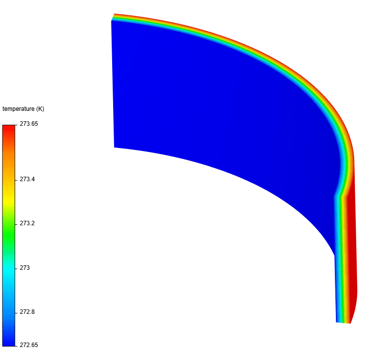
    fixed temperature example results contour plot
    Figure 2: Temperature contour plot of a cylinder subject to fixed temperature values (see validation case below).

    Last updated: September 14th, 2022

    Contents