Porous Media and Porosity Characteristics

Porous media is a bidirectional concept. Whether it is isotropic (3D) or 1D, bidirectional means the flow can pass through opposite directions.

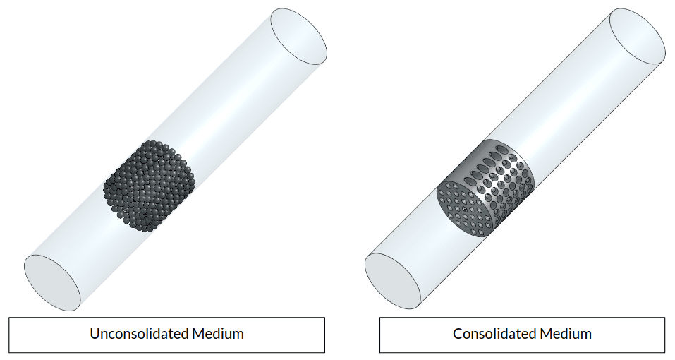
A medium or a material that has voids or pores or is filled with solid particles which let fluid pass through is called a porous medium.

Consolidated medium: The solid body has internal pores. Fluid passes through the pores.

Unconsolidated medium: A pile of solid particles is packed inside a bed. Fluid flows around the particles.

Using porous media simplification reduces CAD and mesh complexity, and saves computational time and expenses.

Consolidated and Unconsolidated Porous Medium — Figure 1: Two types of porous media: Unconsolidated and Consolidated.

With the porous media feature, users can define porosity characteristics of volumes within the computational domain. Defining these porosity characteristics increases the accuracy of certain simulations. SimScale allows its users to model a porous entity inside the simulation domain in five different ways.

A porous media can be created under the Advanced Concepts tab in the simulation tree. The following models are available:

Darcy-Forchheimer Medium

This porosity model takes non-linear effects into account by adding inertial terms to the pressure-flux equation. The model requires both Darcy $d$ and Forchheimer $f$ coefficients to be supplied by the user. If the coefficient f is set to zero, the model degenerates into the Darcy equation.

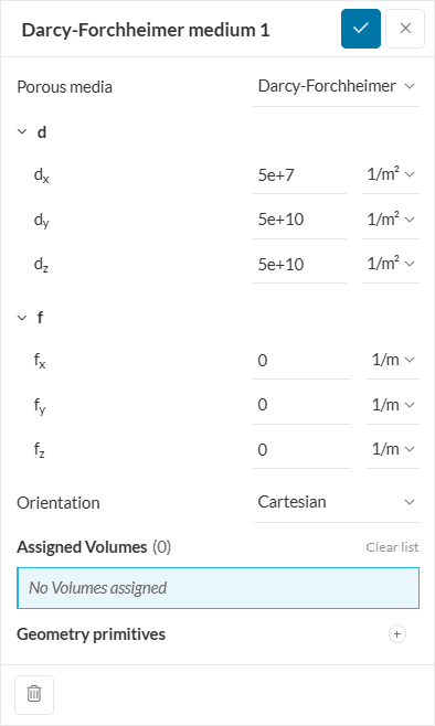
Figure 2: Setup panel for the Darcy-Forchheimer porous model

Furthermore, two-unit vectors for a local coordinate system have to be specified. A third vector is implicitly defined, such that ( $\vec{e_{1}} \vec{e_{2}} \vec{e_{3}}$ ) is a right-handed coordinate system like (x y z). These three vectors should be the main directions of the porous zone resistance. Please note that the $d$ and $f$ coefficients are prescribed for each direction separately. It can be used for both anisotropic and isotropic medium.

The model leads to the following source term for the momentum equation:
$S = - (μ d + \frac{ρ | U |}{2} f) U$
Where:

$S$ can be understood as a pressure gradient $[P a / m]$ ;
μ represents dynamic viscosity $[k g / m . s]$ ;
ρ is the density of the fluid $[k g / m ³]$ ;
$U$ is the velocity of the flow $[m / s]$ .

The Darcy coefficient is the reciprocal of the permeability κ.
$d = \frac{1}{κ}$

Find an example on how to apply the Darcy-Forchheimer model, please check this page.

Fixed Coefficients Medium

This model requires $α$ and $β$ to be supplied by the user. The corresponding source term is:
$S = - ρ_{r e f} (α + β | U |) U$
Where:

$S$ can be understood as a pressure gradient $[P a / m]$ ;
$ρ_{r e f}$ is the density of the fluid $[k g / m ³]$ . This value is only used for compressible and convective heat transfer simulations. Otherwise, the $ρ$ value specified under materials is used;
$U$ is the velocity of the flow $[m / s]$ .

Figure 3: Setup for the Fixed coefficients medium porous model

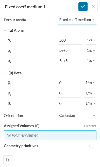
Similarly to the Darcy-Forchheimer model, the user has to specify two unit vectors for a local coordinate system. The $α$ and $β$ coefficients are input based separately for each direction. Therefore, a fixed coefficients medium can be used to define isotropic and non-isotropic porosity.

Once the setup is complete, a porous region must be assigned. Such a region can be defined using geometry primitives or cell zones.

Important

Fixed coefficients, alongside with the pressure loss curve model, are the only two that can be used for compressible, convective heat transfer, and incompressible cases.
The Darcy-Forchheimer, Power Law, and Perforated Plate models should only be used for incompressible and convective heat transfer (with compressibility disabled).

Power Law Medium

In the power law formulation, the source term for the momentum equation is given by:

$S = - ρ C_{0} | U |^{(C_{1})}$
Where:

$S$ can be understood as a pressure gradient $[P a / m]$ ;
$ρ$ is the density of the fluid $[k g / m ³]$ ;
$C_{0}$ is the linear coefficient;
$C_{1}$ is the exponent coefficient;
$U$ is the velocity of the flow $[m / s]$ .

Figure 4: Setup for the Power law porous model

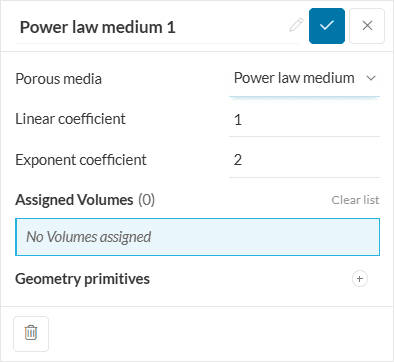
Note that a power law media will always be isotropic. Cell zones and geometry primitives can be used to assign a power law porous media.

For an example on how to apply the power law model, please check this page.

Pressure Loss Curve

The pressure loss curve is a simplified version of the Darcy-Forchheimer model.

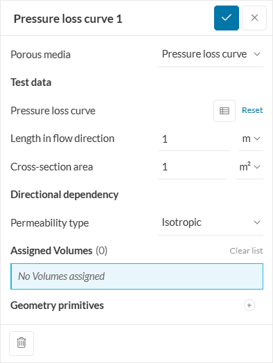
As input, the user has to provide the following information:

A table of volumetric flux $[m ³ / s]$ versus $Δ P [P a]$ for the geometry. A minimum of 3 data points have to be specified. Note: For better results, always start the table by defining a data point (0, 0) in the first line;

specifying data points for porosity documentation case example in simscale platform — Figure 6: Example of data points input. At least 3 data points have to be provided.

Length of the porous media in the flow direction $[m]$ ;
Cross-section area $[m ²]$ .
Permeability type

Important

These inputs define the length of the porous media which was used to generate the curve and its cross-sectional area (normal to flow). They refer to the experimental model’s dimensions, and not to the CAD part that is being used to model the porous media.

Based on the input, a polynomial curve fit is performed and the Darcy-Forchheimer coefficients are automatically calculated. Therefore, the pressure loss curve formulation is a more convenient way of using the Darcy-Forchheimer model.

Important

Curve fitting methods work when a total of three or more data points are provided (including the first [0, 0] point). However, oftentimes, users only have a single non-zero data point for volumetric flux versus $Δ P$ .

In case a single data point is available for your geometry, the approach described below can be used. This approximation is especially good for turbulent flow, providing satisfactory agreement:

1. Following the Darcy-Forchheimer model, assume that the Darcy coefficient is zero. Therefore, only the inertial term (Forchheimer) is considered;

2. Calculate f. Rearranging the Darcy-Forchheimer formulation, we have:
$f = \frac{2 Δ P}{ρ U^{2}}$

3. Extrapolate another data point, by choosing a different velocity (e.g. 2 times greater than the velocity from the first data point) and calculating the corresponding $Δ P$ :
$Δ P = \frac{f ρ U^{2}}{2}$

4. Calculate the corresponding flow rate for the velocity chosen in step 3;

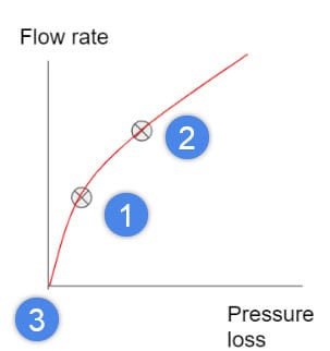
5. The picture below shows the resulting three points. [1] represents the initial data point. [2] is the point that is predicted and [3] is the (0, 0) data point;

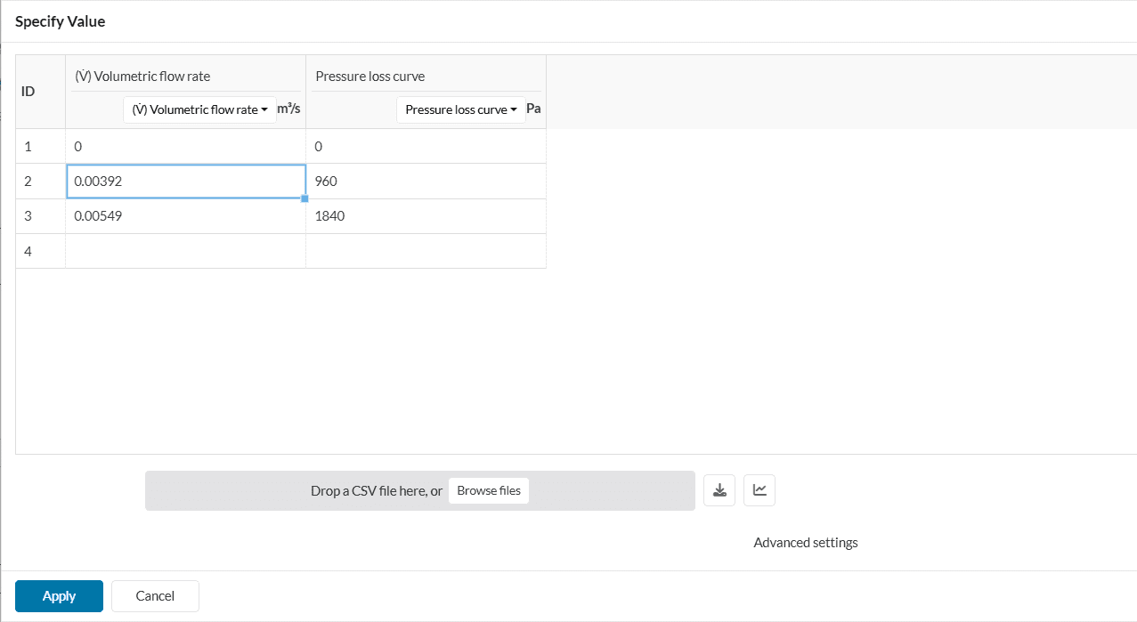
extrapolating data point porous media — Figure 7: Extrapolating one data point for the pressure loss curve model.

6. Input the data points in the table, keeping in mind that the first point should be (0, 0).

7. The table values should have a consistently increasing trend from (0,0) to the maximum point. In addition, the table values should not be repeated.

Perforated Plate

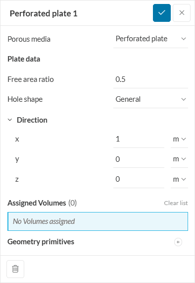
The perforated plate model estimates pressure loss based on geometrical parameters. As inputs, the user has to provide:

Free area ratio: This is a ratio between the open area of the perforated plate (area covered by the holes) and the total area of the plate $(\frac{A_{h}}{A})$ ;
The shape of the hole: Default is a general shape. A circular shape is also available. In case of a circular shape, the average hole diameter should be specified;
Flow direction: With this input, the user can specify the principal flow direction within the medium. This direction is based on global coordinates.

The perforated plate model is based on the formulation presented in [1].

Figure 8: Setup panel for Perforated plate porous model

Important

For all porous media models, it’s important to refine the region around the porous media appropriately.
Make sure at least 5 mesh cells are placed across the porous media thickness.

Pressure Loss Function

The pressure loss function porous media is exclusive to the multi-purpose solver. Similarly to the pressure loss curve model, the user defines a volumetric flow rate versus delta pressure table by clicking on the table button:

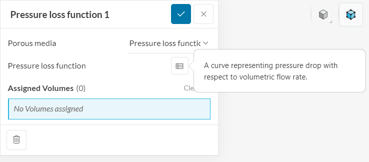
At least 3 data points are recommended for the table definition, with the first one being 0 flow rate and 0 pressure drop. With more points a better interpolation is obtained.

Note that this porous media model is always isotropic and the volume assignment needs to be done to a CAD volume since geometry primitives are not supported.

Darcy Law Medium

The Darcy Law medium is another porous media model exclusive to the multi-purpose solver. With the current implementation, this porous media model is always isotropic.

The Darcy Law medium in SimScale is based on the following formulation:

$d P = \frac{μ L U}{K} + \frac{C_{d} ρ L U^{2}}{\sqrt{K}}$

Where:

$d P$ is a pressure gradient $[P a]$ ;
$μ$ is the dynamic viscosity of the fluid $[k g / m . s]$ ;
$L$ is the length of the porous media in the flow direction;
$U$ is the velocity of the flow $[m / s]$ ;
$K$ is the permeability coefficient $[1 / m^{2}]$ ;
$C_{d}$ is the drag coefficient;
$ρ$ is the density of the fluid $[k g / m ³]$ .

darcy law medium porous media in SimScale — Figure 10: Setup for Darcy Law medium porous model

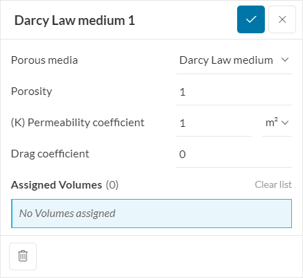
When inspecting the formulation that is used for the Darcy Law medium model, when the drag coefficient $C_{d}$ term is not zero, both Darcy (linear) and Forchheimer (quadratic) terms will be present. This is usually the case for applications involving larger velocities since the quadratic term becomes more relevant as velocity increases.

On the other hand, when $C_{d}$ is zero, this model is purely based on Darcy’s law.

References

VDI Heat Atlas. Second Edition. Springer-Verlag Berlin Heidelberg 2010.

Last updated: February 25th, 2025

Did this article solve your issue?

How can we do better?

We appreciate and value your feedback.

What's Next

Power Source

part of: Advanced Concepts

Porous Media and Porosity Characteristics

Darcy-Forchheimer Medium

Fixed Coefficients Medium

Power Law Medium

Pressure Loss Curve

Perforated Plate

Pressure Loss Function

Darcy Law Medium

Did this article solve your issue?

How can we do better?

Contents