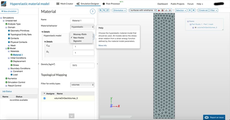
Hyperelastic material models are regularly used to represent the large deformation behavior of materials with FEA. They are commonly used to model mechanical behaviors of unfilled/filled elastomers. In addition to elastomers, hyperelastic material models are also used to approximate the material behavior of biological tissues, polymeric foams, etc.
Linearly elastic materials are described through two material constants (like Young’s modulus and Poisson ratio). In contrast, hyperelastic materials are described through a strain-energy density function. The strain-energy density can be used to derive a nonlinear constitutive model (i.e., stresses as a function of large strain deformation measures like deformation gradient or Cauchy-Green tensors, etc.). There are several models proposed in the literature such as the Neo-Hookean, Mooney-Rivlin and Signorini models, which are available on the SimScale cloud-based CAE platform, as well as Ogden, Yeoh, Arruda-Boyce, which are not available on SimScale. A detailed mathematical description of these hyperelastic, strain-energy density functions can be found in the SimScale documentation.

The Signorini hyperelastic material model can be described as a more generalized version of the Mooney-Rivlin model. A detailed description of validation of the available models for uniaxial, equibiaxial, and pure shear can be found on the SimScale website.
The purpose of a helmet is to protect the person who wears it from a head injury during impact. In this project, the impact of a human skull with and without a helmet was simulated with a nonlinear dynamic analysis. Download this case study for free.
Hyperelastic Material Effect of Temperature
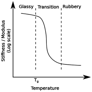
In general, elastomers demonstrate a strong dependence on the strain rate, temperature, and loading history. Their mechanical behavior can be separated into three regimes: glassy (and brittle), viscoelastic, and rubbery. As shown in Fig. 02 below, at a particular temperature, known as the glass transition temperature, the behavior is glassy (and brittle) in nature. At temperatures above it, the behavior changes to viscoelastic and can further shift to rubbery.

Hyperelastic material models are ideally suited to describing the rubbery phase of elastomeric behavior. In this phase, the material can be assumed to be independent of loading history and temperature, and it displays the pure elastic response.
Tip 01: “What is the glass transition temperature of the elastomer being modeled?” If the working temperature is significantly higher than the glass transition temperature of the elastomer, then the hyperelastic material model could be used in your FEA.
Hyperelastic Material Parameter Identification
In large deformation mechanics, it is important to be certain of what stress measures are being used. Unlike in linear elasticity, while using hyperelastic models, the undeformed (or reference) and deformed (or current) configurations need to be distinguished and addressed. For example, during a uniaxial tensile test, the area of the specimen is measured prior to the test (i.e., in the undeformed configuration) and the force is measured as the test progresses (i.e., in the deformed configuration). Thus, the “stress” plotted in the stress-strain curve obtained experimentally is the first Piola-Kirchhoff (or Nominal) stress.

As illustrated in the strain-energy density function, each hyperelastic material model requires one or more material parameters to be identified from experiments. Some of the commonly used experiments are uniaxial tensile test, equibiaxial tensile test, and shear (or planar) test. Fig. 03 shows the fitting using all three of these experiments. A good rule of thumb is one experiment for each parameter being used by the model. Fitting parameters for a Mooney-Rivlin model with only one experiment, like the uniaxial tensile test, could lead to non-uniqueness of parameters (i.e., the fitting procedure can lead to different parameters based on different starting approximations).
Tip 02: “What experimental data is available for parameter fitting?” For a unique set of parameters, just one experiment would be sufficient to obtain parameters for Neo-Hookean; at least two experiments for Mooney-Rivlin; three for Signorini/Arruda-Boyce; and three or more for Ogden models.
Hyperelastic Material Magnitude of Deformation
The next step would be to identify the magnitude of deformation (or strain) that the component would be subjected to. For example, rubber components are commonly used to suppress vibrations. In cases where the deformations are moderate (<100%), simple models like Neo-Hookean would suffice. Such a simplification can be invaluable in reducing the computational effort.

As illustrated in Fig. 04, Treloar experimental data is compared with different hyperelastic models. A useful rule of thumb is that the Ogden model (of order 3) is the most suitable for the entire range (0% up to failure). While Neo-Hookean model performs well up to 100%, Mooney-Rivlin is best up to 150-200%. In contrast, the Yeoh and Arruda-Boyce models are most suitable when fitted for the range of usage.
Tip 03: “What is the magnitude of deformation (in comparison to its size) that is experienced by the component?” Up to 100% (Neo-Hookean); 150-200% (Mooney-Rivlin); 0-Failure (Full Ogden); particular range of a-b (Yeoh or Arruda-Boyce).
Material Stability Stability of Hyperelastic Material Models
As previously discussed, it is possible that models with multiple parameters can be fitted with just one experiment. In such a case, depending on the material parameters obtained, the model can be always or conditionally stable or unstable (for other loading conditions).
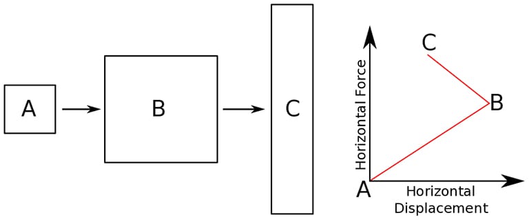
The Mooney-Rivlin hyperelastic material model (with a polynomial of order one) demonstrates an instability when subjected to biaxial loads. The strain level at which an instability occurs depends on the ratio of C01/C10. If the ratio C01/C10 is decreased, the biaxial strain corresponding to instability increases. For example, for C01 = 1/8 and C10 = 1/24 and application of equibiaxial loading, an instability set at an extension of about 1.6. As shown in Fig. 05, upon application of equibiaxial load, the body moves from state A to B. Now, at state B, as the horizontal force is increased with constant vertical force, the body reaches state C. This is an unphysical response where the displacement decreases as force increases.

In contrast, the stability of the Ogden model depends on the chosen parameters, whereas the Neo-Hookean model is always stable.
Tip 04: “Do the chosen parameters lead to stable behavior in the range of usage?” If the fitting is done using a particular test type(s), then it would be useful to try other tests to check the stability of the model parameter(s).
Material Parameters Consistency of Parameters Used in FEA
With regard to Neo-Hookean, Mooney-Rivlin, and Signorini models, for consistency with linear elasticity, the material parameters need to satisfy the following conditions:
- G = 2 (C10 + C01), where G is the shear modulus
- D1 = K/2, where K is the bulk modulus
Additionally, it is necessary to note that, as the Poisson ratio approaches 0.5 (once >0.4), more complicated formulations are necessary to account for the incompressible behavior. The stresses measured in experiments using models that support incompressibility are typically much higher than the results obtained from compressible models. This shall be discussed in a future post, along with meshing issues related to modeling hyperelastic/incompressible materials with FEA.
Tip 04: “Do you really need an incompressible model?” Compressible models can significantly underestimate the stresses calculated with an FEA. Instead, try using SimScale’s reduced integration option available in the mesh tree. Alternatively, elements with mixed or enhanced formulations that are more accurate may become available in the future.
I hope this article has answered your questions regarding how to choose hyperelastic material models for an finite element analysis (FEA). If you’d like to put your knowledge into practice, SimScale offers the possibility to carry out simulations 100% in a web browser. Just create a free Community account here.
Additionally, watch the recording of a webinar in partnership with Onshape about medical devices design optimization with cloud-based CAD and CAE. All you need to do is fill out this short form and it will play automatically.


